Limit Theorems of Random Variables
Many practical situations involve random variables that are defined as the sum or average of other random variables. For instance, estimating a population mean from a sample mean relies heavily on the properties of these sums. Limit theorems provide the mathematical foundation for such estimations.
Limit theorems are fundamental results in probability theory that describe the behavior of sums of random variables as the number of terms increases. We will focus on two key theorems:
Limit theorems are fundamental results in probability theory that describe the behavior of sums of random variables as the number of terms increases. We will focus on two key theorems:
- The Law of Large Numbers (LLN): this theorem explains why averages stabilize. It states that as you perform an experiment many times, the average of the results (experimental mean) gets closer and closer to the expected value (theoretical mean).
- The Central Limit Theorem (CLT): this theorem explains the shape of the distribution. It states that if you sum a large number of independent random variables, the distribution of their sum (or mean) tends toward a normal distribution, regardless of the original distribution of the variables (under mild technical conditions).
- Does the experimental probability (or observed frequency) approach the theoretical probability as the number of trials increases? Yes, the Law of Large Numbers guarantees this.
- Can we quantify the error between our sample estimate and the true value? Yes, the Central Limit Theorem allows us to define confidence intervals and error margins using the normal distribution.
Linear Combination of Random Variables
Consider flipping a fair coin two times. Let the random variables \(X_1\) and \(X_2\) represent the outcome of the first and second coin flips, respectively. We code success (Heads) as 1 and failure (Tails) as 0. We assume the two flips are independent.
Thus, \(X_1\) and \(X_2\) follow a Bernoulli distribution with probability of success \(p=\dfrac{1}{2}\). We are interested in two new random variables:
Thus, \(X_1\) and \(X_2\) follow a Bernoulli distribution with probability of success \(p=\dfrac{1}{2}\). We are interested in two new random variables:
- \(S_2 = X_1 + X_2\): the total number of heads.
- \(\overline{X}_2 = \dfrac{X_1 + X_2}{2}\): the average proportion of heads.
- Probability distribution: We can visualize the outcomes using a probability tree.
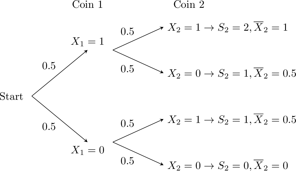
\quad\(s\) (Sum) \(0\) \(1\) \(2\) \(P(S_2=s)\) \(1/4\) \(1/2\) \(1/4\) \(\bar{x}\) (Mean) \(0\) \(0.5\) \(1\) \(P(\overline{X}_2=\bar{x})\) \(1/4\) \(1/2\) \(1/4\) - Expectation:$$E(S_2) = 0\left(\tfrac{1}{4}\right) + 1\left(\tfrac{1}{2}\right) + 2\left(\tfrac{1}{4}\right) = 1,$$$$E(\overline{X}_2) = 0\left(\tfrac{1}{4}\right) + 0.5\left(\tfrac{1}{2}\right) + 1\left(\tfrac{1}{4}\right) = 0.5.$$
- Connection to individual variables:
Since \(E(X_1) = E(X_2) = p = 0.5\), we have:$$E(S_2) = 1 = 2 \times 0.5 = 2E(X_1),$$$$E(\overline{X}_2) = 0.5 = E(X_1).$$ - Variance:$$V(S_2) = (0-1)^2\left(\tfrac{1}{4}\right) + (1-1)^2\left(\tfrac{1}{2}\right) + (2-1)^2\left(\tfrac{1}{4}\right) = \tfrac{1}{4} + 0 + \tfrac{1}{4} = 0.5,$$$$V(\overline{X}_2) = (0-0.5)^2\left(\tfrac{1}{4}\right) + (0.5-0.5)^2\left(\tfrac{1}{2}\right) + (1-0.5)^2\left(\tfrac{1}{4}\right) = \tfrac{0.25}{4} + 0 + \tfrac{0.25}{4} = 0.125.$$
- Connection to individual variance:
Since \(V(X_1) = p(1-p) = 0.25\), it follows that:$$V(S_2) = 0.5 = 2 \times 0.25 = 2V(X_1),$$$$V(\overline{X}_2) = 0.125 = \frac{0.25}{2} = \frac{V(X_1)}{2}.$$
Definition Linear Combination of Random Variables
A linear combination of random variables \(X_1, X_2, \ldots, X_n\) is a new random variable \(Y\) defined as$$ Y = a_1 X_1 + a_2 X_2 + \ldots + a_n X_n, $$where \(a_1, a_2, \ldots, a_n\) are constant coefficients.
Definition Sum and Mean of Random Variables
Given \(n\) random variables \(X_1, X_2, \dots, X_n\):
- The sum is denoted \(S_n = X_1 + X_2 + \ldots + X_n\).
- The sample mean is denoted \(\overline{X}_n = \dfrac{X_1 + X_2 + \ldots + X_n}{n}\).
Proposition Properties of Expectation and Variance
For random variables \(X_1, \dots, X_n\) and constants \(a_1, \dots, a_n\):
- Expectation is linear: $$ E\left(\sum_{i=1}^n a_i X_i\right) = \sum_{i=1}^n a_i E(X_i). $$
- Variance adds for independent variables: if \(X_1, \dots, X_n\) are independent, $$ V\left(\sum_{i=1}^n a_i X_i\right) = \sum_{i=1}^n a_i^2 V(X_i). $$
Proposition Expectation of Sums and Means
If \(X_1, X_2, \dots, X_n\) are identically distributed with mean \(\mu\), then:$$ E(S_n) = n\mu \qquad\text{and}\qquad E(\overline{X}_n) = \mu. $$
- For the sum \(S_n\):
Using linearity of expectation,$$ \begin{aligned}E(S_n) &= E(X_1 + X_2 + \dots + X_n) \\ &= E(X_1) + E(X_2) + \dots + E(X_n) \\ &= \mu + \mu + \dots + \mu \quad \text{(\(n\) times)} \\ &= n\mu.\end{aligned} $$ - For the mean \(\overline{X}_n\):
Using \(E(aX) = aE(X)\),$$ \begin{aligned}E(\overline{X}_n) &= E\left(\frac{S_n}{n}\right) \\ &= \frac{1}{n} E(S_n) \\ &= \frac{1}{n} (n\mu) \\ &= \mu.\end{aligned} $$
Example
Let \(X_1, \dots, X_9\) be random variables with mean \(\mu=5\). Find the expected value of their sum \(S_9\).
$$ E(S_9) = 9 \times \mu = 9 \times 5 = 45. $$
Proposition Variance of Sums and Means
If \(X_1, X_2, \dots, X_n\) are independent and identically distributed with variance \(\sigma^2\) (and standard deviation \(\sigma\)), then:
- For the sum: $$ V(S_n) = n\sigma^2 \quad \text{and} \quad \sigma(S_n) = \sigma\sqrt{n}; $$
- For the mean: $$ V(\overline{X}_n) = \frac{\sigma^2}{n} \quad \text{and} \quad \sigma(\overline{X}_n) = \frac{\sigma}{\sqrt{n}}. $$
- For the sum \(S_n\):
Since the variables \(X_1, \dots, X_n\) are independent, the variance of the sum is the sum of the variances:$$ \begin{aligned}V(S_n) &= V(X_1 + X_2 + \dots + X_n) \\ &= V(X_1) + V(X_2) + \dots + V(X_n) \\ &= \sigma^2 + \sigma^2 + \dots + \sigma^2 \quad \text{(\(n\) times)} \\ &= n\sigma^2.\end{aligned} $$The standard deviation is the square root of the variance:$$ \sigma(S_n) = \sqrt{V(S_n)} = \sqrt{n\sigma^2} = \sigma\sqrt{n}. $$ - For the mean \(\overline{X}_n\):
Using the property \(V(aX) = a^2V(X)\) with \(a = \dfrac{1}{n}\),$$ \begin{aligned}V(\overline{X}_n) &= V\left(\frac{S_n}{n}\right) \\ &= \left(\frac{1}{n}\right)^2 V(S_n) \\ &= \frac{1}{n^2} (n\sigma^2) \\ &= \frac{\sigma^2}{n}.\end{aligned} $$Thus,$$ \sigma(\overline{X}_n) = \sqrt{V(\overline{X}_n)} = \sqrt{\frac{\sigma^2}{n}} = \frac{\sigma}{\sqrt{n}}. $$
Example Sample Proportion
Items coming off an assembly line are defective with probability \(p\). Let \(X_i\) be an indicator variable where \(X_i=1\) if the \(i\)-th item is defective and \(0\) otherwise. Then \(X_i\) follows a Bernoulli distribution. Find the mean and standard deviation of the sample proportion \(\overline{X}_n\).
For a Bernoulli variable, \(\mu = p\) and \(\sigma = \sqrt{p(1-p)}\). Therefore, for the sample mean \(\overline{X}_n\):$$ E(\overline{X}_n) = p, $$$$ \sigma(\overline{X}_n) = \frac{\sigma}{\sqrt{n}} = \sqrt{\frac{p(1-p)}{n}}. $$
Law of Large Numbers
The Law of Large Numbers (LLN) describes the result of performing the same experiment a large number of times. It states that the average of the results obtained from many trials should be close to the expected value and tends to become closer as more trials are performed.
In practice, this justifies our intuition that experimental probability estimates theoretical probability. While short-term results are unpredictable (for example, a casino might lose money on a single spin), long-term averages are highly predictable (in the long run, the casino wins).
In practice, this justifies our intuition that experimental probability estimates theoretical probability. While short-term results are unpredictable (for example, a casino might lose money on a single spin), long-term averages are highly predictable (in the long run, the casino wins).
Definition Limit Mean
If the limit exists, we denote the limit of the sample mean as \(n\) approaches infinity by \(\overline{X}_\infty\):$$ \overline{X}_\infty = \lim_{n\to\infty} \overline{X}_n. $$
Theorem Law of Large Numbers
For independent, identically distributed random variables \(X_1, X_2, \dots\) with mean \(\mu\) and standard deviation \(\sigma\), the sample mean converges to the population mean as the number of observations goes to infinity. In more advanced notation,$$ P\!\big(\overline{X}_\infty = \mu\big) = 1. $$This means that the sample mean converges to the population mean with (probabilistic) certainty.
Recall that the variance of the sample mean is$$ V(\overline{X}_n) = \frac{\sigma^2}{n}. $$As \(n \to \infty\), the term \(\dfrac{\sigma^2}{n}\) approaches \(0\).
A random variable with variance \(0\) has no dispersion; it is almost surely constant. Therefore, as \(n\) grows, the distribution of \(\overline{X}_n\) becomes more and more concentrated around its expected value \(\mu\), and in the limit it collapses to this single value.
A random variable with variance \(0\) has no dispersion; it is almost surely constant. Therefore, as \(n\) grows, the distribution of \(\overline{X}_n\) becomes more and more concentrated around its expected value \(\mu\), and in the limit it collapses to this single value.
The limiting distribution is deterministic: in the limit the sample mean takes the value \(\mu\) with probability \(1\).
Example Experimental vs Theoretical Probability
Consider tossing a cone. The probability \(p\) of it landing on its base is not known a priori.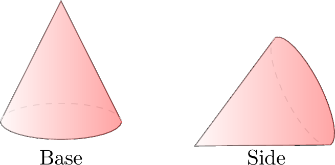
In practice, we can never repeat an experiment infinitely many times. The sample mean is always an approximation of the true mean. The next theorem, the Central Limit Theorem, allows us to quantify the error of this approximation and to describe how the sample mean fluctuates around \(\mu\) for large but finite \(n\).
Central Limit Theorem
The Central Limit Theorem (CLT) is one of the most remarkable results in mathematics. Informally, it states that if you take a sufficiently large sample size from a population with any distribution (not necessarily normal), the distribution of the sample mean (or sum) is approximately normal.
This normal approximation is what justifies using the normal distribution to build confidence intervals and perform hypothesis tests, even when the underlying population is not itself normal.
This normal approximation is what justifies using the normal distribution to build confidence intervals and perform hypothesis tests, even when the underlying population is not itself normal.
Proposition Sum and Mean of Normal Variables
If \(X_1, \dots, X_n\) are independent and normally distributed with mean \(\mu\) and standard deviation \(\sigma\), then:
- The sum \(S_n\) is exactly normally distributed with mean \(n\mu\) and variance \(n\sigma^2\): $$ S_n \sim N(n\mu, n\sigma^2). $$
- The sample mean \(\overline{X}_n\) is exactly normally distributed with mean \(\mu\) and variance \(\dfrac{\sigma^2}{n}\): $$ \overline{X}_n \sim N\!\left(\mu, \frac{\sigma^2}{n}\right). $$
Example
Let \(X_1, \dots, X_5\) be normally distributed random variables with mean \(90\) and standard deviation \(20\).
- Is \(\overline{X}_5\) normally distributed?
- Find \(P(80 \leqslant \overline{X}_5 \leqslant 100)\).
- Yes, because any linear combination of normal variables is also normal. In particular, the mean \(\overline{X}_5\) is normally distributed.
- The mean of \(\overline{X}_5\) is \(E(\overline{X}_5) = 90\). Its standard deviation is $$ \sigma(\overline{X}_5) = \frac{20}{\sqrt{5}} \approx 8.94. $$ Using a normal distribution calculator for \(N(90, 8.94^2)\), we obtain $$P(80 \leqslant \overline{X}_5 \leqslant 100) \approx 0.737.$$
Proposition Standardized Mean
For \(n\) independent random variables with common mean \(\mu\) and standard deviation \(\sigma\), the sample mean \(\overline{X}_n\) has$$ E(\overline{X}_n) = \mu, \qquad \sigma(\overline{X}_n) = \frac{\sigma}{\sqrt{n}}. $$The standardized variable$$ Z_n = \frac{\overline{X}_n - \mu}{\sigma/\sqrt{n}} $$has mean \(0\) and standard deviation \(1\).
First, recall the properties of the sample mean \(\overline{X}_n\):$$ E(\overline{X}_n) = \mu \quad \text{and} \quad \sigma(\overline{X}_n) = \frac{\sigma}{\sqrt{n}}. $$
- Mean of \(Z_n\):
Using linearity of expectation, \(E(aX+b) = aE(X)+b\):$$ \begin{aligned}E(Z_n) &= E\left(\frac{\overline{X}_n - \mu}{\sigma/\sqrt{n}}\right) \\ &= \frac{1}{\sigma/\sqrt{n}} \left( E(\overline{X}_n) - \mu \right) \\ &= \frac{1}{\sigma/\sqrt{n}} (\mu - \mu) \\ &= 0.\end{aligned} $$ - Standard deviation of \(Z_n\):
Using the property \(\sigma(aX+b) = |a|\sigma(X)\):$$ \begin{aligned}\sigma(Z_n) &= \sigma\left(\frac{\overline{X}_n - \mu}{\sigma/\sqrt{n}}\right) \\ &= \frac{1}{\sigma/\sqrt{n}} \cdot \sigma(\overline{X}_n) \\ &= \frac{1}{\sigma/\sqrt{n}} \cdot \frac{\sigma}{\sqrt{n}} \\ &= 1.\end{aligned} $$
The power of the Central Limit Theorem is especially visible when we start from a distribution that is not normal. For example, suppose each \(X_i\) follows a uniform distribution. The figures below show the density of the standardized sum (or mean) \(Z_n\) for increasing \(n\).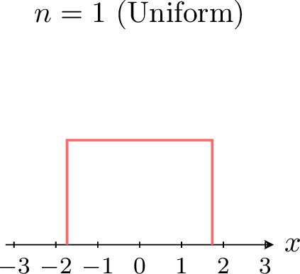 \(\quad\)
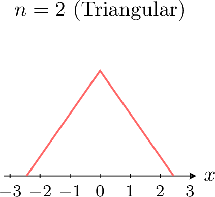 \(\quad\)
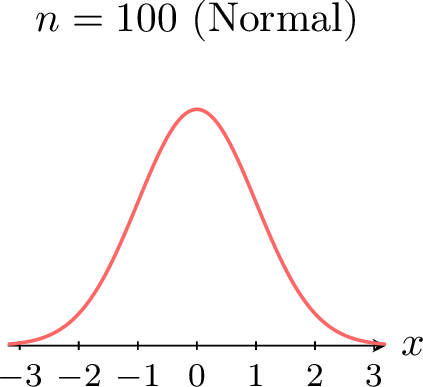
\(\quad\)\(\quad\)
Theorem Central Limit Theorem
Let \(X_1, X_2, \dots, X_n\) be independent, identically distributed random variables with mean \(\mu\) and standard deviation \(\sigma\). If the sample size \(n\) is sufficiently large (typically \(n \ge 30\)), then:
- The sample mean \(\overline{X}_n\) is approximately normally distributed: $$ \overline{X}_n \approx N\!\left(\mu, \frac{\sigma^2}{n}\right). $$
- The sum \(S_n\) is approximately normally distributed: $$ S_n \approx N(n\mu, n\sigma^2). $$
- The standardized variable $$ Z_n = \frac{\overline{X}_n - \mu}{\sigma/\sqrt{n}} $$ is approximately distributed as a standard normal \(N(0,1)\) for large \(n\). More rigorously, the distribution of \(Z_n\) converges to \(N(0,1)\) as \(n \to \infty\).
Example
A population of random variables has mean \(174\) and standard deviation \(6\). A sample of size \(64\) is taken.
- Is the sample mean \(\overline{X}_{64}\) approximately normally distributed? Explain.
- Find the mean and standard deviation of \(\overline{X}_{64}\).
- Find the probability that the sample mean is between \(172\) and \(176\).
- Yes. Since the sample size is \(n=64\) (which is large, \(n \ge 30\)), the Central Limit Theorem applies, and the sampling distribution of \(\overline{X}_{64}\) is approximately normal.
- Mean and standard deviation: $$ E(\overline{X}_{64}) = \mu = 174, $$ $$ \sigma(\overline{X}_{64}) = \frac{\sigma}{\sqrt{n}} = \frac{6}{\sqrt{64}} = \frac{6}{8} = 0.75. $$
- Using a normal distribution calculator with \(\mu=174\) and \(\sigma=0.75\): $$ P(172 \leqslant \overline{X}_{64} \leqslant 176) \approx 0.9923. $$