Continuous Random Variables
Consider a random experiment where a spinner is spun, and the continuous random variable \(X\) represents the angle spun, measured in degrees over the interval \([0, 360)\).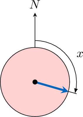
Definitions
Continuous Random Variable
Definition Continuous Random Variable
A random variable is continuous if its set of possible values is an entire interval of real numbers. A continuous random variable can take any value within its range, meaning there is an infinite number of possibilities.
Probability Density Function
A probability density function describes the likelihood of a continuous random variable taking values within a specific range. Unlike discrete random variables, where probabilities are assigned to individual outcomes, continuous variables use the pdf to compute probabilities over intervals via integration.
Definition Probability Density Function
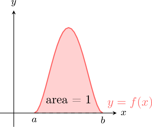
A function \(f\) is a probability density function (pdf) on the interval \([a, b]\) if:
- \(f(x) \geq 0\) for all \(x \in [a, b]\) (non-negative everywhere),
- \(\int_{a}^{b} f(x) \, dx = 1\) (the total area under the curve equals 1).
Example
The random variable \(X\) takes values on \([0, 2]\) with density \(f(x) = \frac{x}{2}\).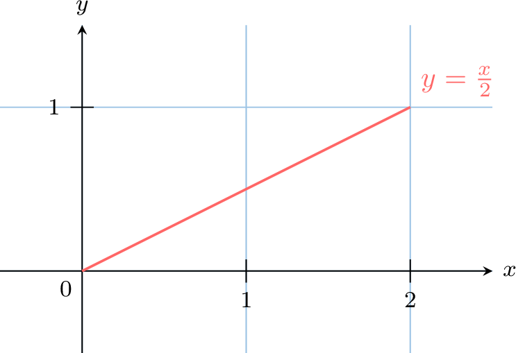
- \(f(x) = \frac{x}{2} \geq 0\) for all \(x \in [0,2]\), since \(x \geq 0\).
- Compute the total area: $$ \begin{aligned}[t] \int_{0}^{2} f(x) \, dx &= \int_{0}^{2} \frac{x}{2} \, dx \\ &= \left[ \frac{x^2}{4} \right]_{0}^{2} \\ &= \frac{2^2}{4} - 0 = 1 \end{aligned} $$ Since both conditions hold, \(f(x) = \frac{x}{2}\) is a valid pdf on \([0, 2]\).
Definition Density of a Continuous Random Variable
A random variable \(X\) with values on \([a, b]\) has a density \(f\), if the probability that \(X\) lies between \(c\) and \(d\) (\(c, d \in [a, b]\)) is:$$P(c \leq X \leq d) = \int_{c}^{d} f(x) \, dx$$This represents the area under the curve \(y = f(x)\) from \(x = c\) to \(x = d\).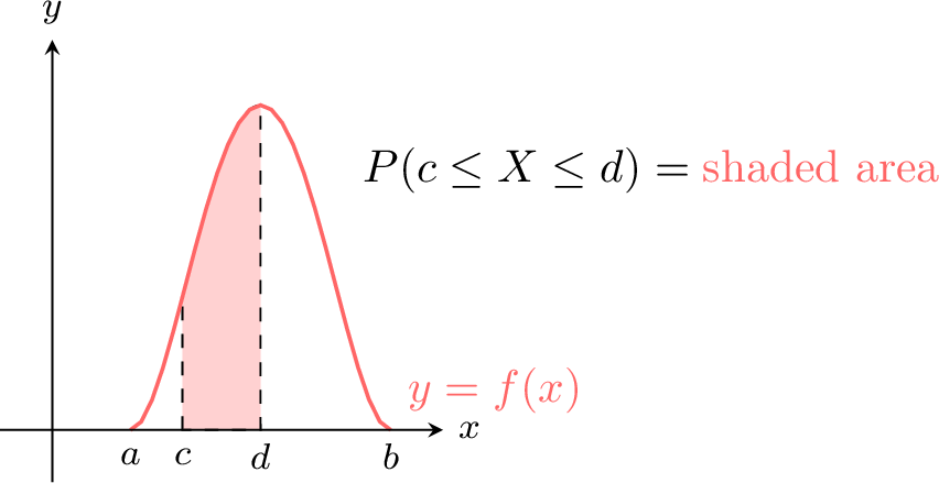
Remark
- Since \(f(x) \geq 0\), \(P(c \leq X \leq d) \geq 0\).
- Since \(\int_{a}^{b} f(x) \, dx = 1\), \(P(a \leq X \leq b) = 1\).
Example
The random variable \(X\) with values on \([0, 2]\) has density \(f(x) = \frac{x}{2}\). Find \(P(1 \leq X \leq 2)\).
$$\begin{aligned}[t]P(1 \leq X \leq 2) &= \int_{1}^{2} \frac{x}{2} \, dx \\
&= \left[ \frac{x^2}{4} \right]_{1}^{2} \\
&= \frac{2^2}{4} - \frac{1^2}{4} \\
&= 1 - \frac{1}{4}\\
&= \frac{3}{4}\end{aligned}$$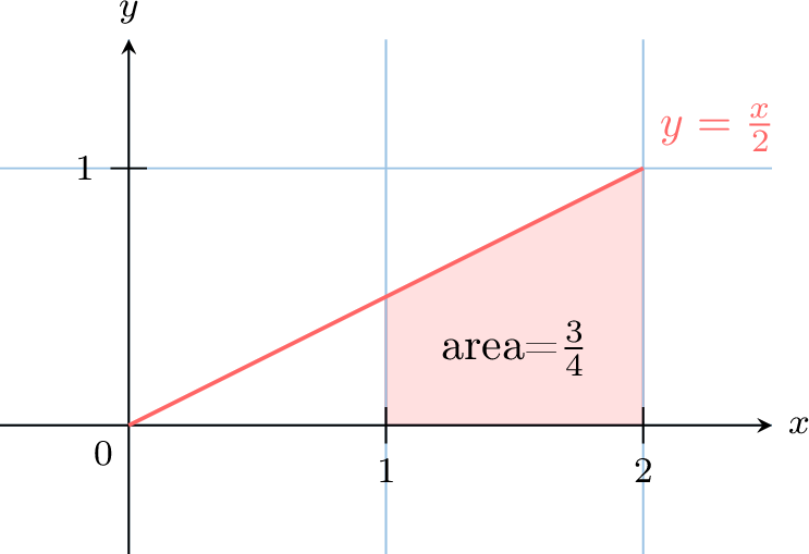
Expectation
The expectation (or expected value) of a continuous random variable is the "average" value it would take if the experiment were repeated infinitely. It represents the center of the distribution and is calculated as a weighted average, where the pdf \(f(x)\) provides the weighting:$$\begin{aligned}[t]E(X)&=\sum_{x\in[a,b]}x P(x \leqslant X < x+\mathrm d x)\\
&=\sum_{x\in[a,b]}x \dfrac{P(x \leqslant X < x+\mathrm d x)}{\mathrm d x}\mathrm d x\\
&=\int_{a}^b xf(x)\;\mathrm d x\\
\end{aligned}$$
Definition Expectation
For a continuous random variable \(X\) with density \(f\) on \([a, b]\), the expected value is $$E(X) = \int_{a}^{b} x f(x) \, dx.$$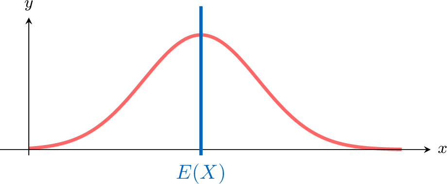
Example
The random variable \(X\) with values on \([0, 3]\) has density \(f(x) = \frac{x^2}{9}\):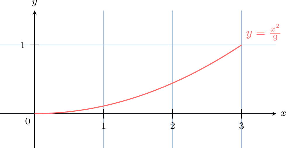
Compute \(E(X)\): $$ \begin{aligned}[t] E(X) &= \int_{0}^{3} x \cdot \frac{x^2}{9} \, dx \\
&= \int_{0}^{3} \frac{x^3}{9} \, dx \\
&= \left[ \frac{x^4}{36} \right]_{0}^{3} \\
&= \frac{3^4}{36} - 0 \\
&= 2.25 \end{aligned} $$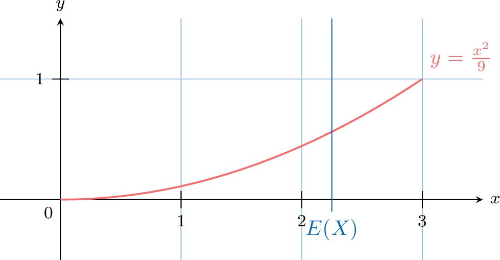
Example
The random variable \(X\) with values on \([0,2]\) has density \(f(x) = \frac{x}{2}\):
Compute \(E(X)\):$$\begin{aligned}[t]E(X) &= \int_{0}^{2} x \cdot \frac{x}{2} \, dx \\
&= \int_{0}^{2} \frac{x^2}{2} \, dx \\
&= \left[ \frac{x^3}{6} \right]_{0}^{2} \\
&= \frac{2^3}{6} - 0 \\
&= \frac{8}{6} \\
&= \frac{4}{3} \\
\end{aligned}$$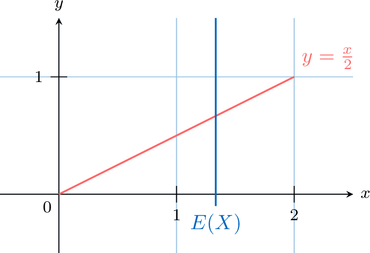
Variance
The variance of a continuous random variable measures the spread of its values around the expected value if the experiment were repeated infinitely. It quantifies the distribution’s dispersion and can be calculated as for a discrete random variable:$$\begin{aligned}[t]V(X) &= \sum_{x \in [a, b]} (x - E(X))^2 P(x \leq X < x + dx) \\
&= \sum_{x \in [a, b]} (x - E(X))^2 \frac{P(x \leq X < x + dx)}{dx} \cdot dx \\
&= \int_{a}^{b} (x - E(X))^2 f(x) \, dx\end{aligned}$$
Definition Variance and Standard Deviation
For a continuous random variable \(X\) with density \(f\) on \([a, b]\), the variance is$$V(X) = \int_{a}^{b} (x - E(X))^2 f(x) \, dx.$$The standard deviation is$$\sigma = \sqrt{V(X)}.$$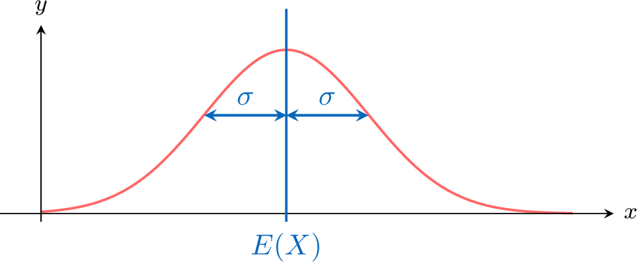
Proposition Computational Formula for Variance
A more convenient formula for variance computation is:$$V(X) = E(X^2) - [E(X)]^2$$
Example
The random variable \(X\) with values on \([0,2]\) has density \(f(x) = \frac{x}{2}\).
Find \(V(X)\).
Find \(V(X)\).
- Compute \(E(X)\): $$ \begin{aligned}[t] E(X) &= \int_{0}^{2} x \cdot \frac{x}{2} \, dx \\ &= \int_{0}^{2} \frac{x^2}{2} \, dx \\ &= \left[ \frac{x^3}{6} \right]_{0}^{2} \\ &= \frac{2^3}{6} - 0 \\ &= \frac{8}{6} \\ &= \frac{4}{3} \\ \end{aligned} $$
- Compute \(\int_{0}^{2} x^2 \cdot f(x) \, dx\): $$ \begin{aligned}[t] \int_{0}^{2} x^2 \cdot f(x) \, dx &=\int_{0}^{2} x^2 \cdot \frac{x}{2} \, dx\\ &= \int_{0}^{2} \frac{x^3}{2} \, dx \\ &= \left[ \frac{x^4}{8} \right]_{0}^{2} \\ &= \frac{2^4}{8} - 0 \\ &= \frac{16}{8} \\ &= 2 \end{aligned} $$
- Compute \(V(X)\) using the alternative formula: $$ \begin{aligned}[t] V(X) &= \int_{0}^{2} x^2 \cdot f(x) \, dx - [E(X)]^2 \\ &= 2 - \left(\frac{4}{3}\right)^2 \\ &= 2 - \frac{16}{9} \\ &= \frac{18}{9} - \frac{16}{9} \\ &= \frac{2}{9} \end{aligned} $$
Continuous Uniform Distribution
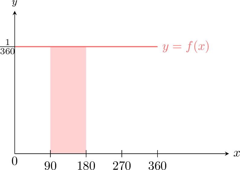
The continuous uniform distribution applies to events that are equally likely across an interval, such as the spinner example. The density is constant over the range.
Definition Continuous Uniform Distribution
A continuous random variable \(X\) follows a continuous uniform distribution on \([a, b]\) if its density is:$$f(x) = \frac{1}{b - a} \quad \text{for} \quad a \leq x \leq b$$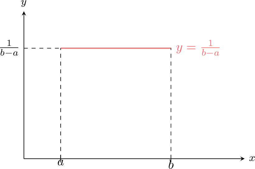
Proposition Properties
Let \( X \) be a continuous random variable following a continuous uniform distribution on \([a, b]\):
- for all \( c, d \in [a, b] : P(c \leq X \leq d) = \frac{d - c}{b - a}\),
- \(E(X) = \frac{a + b}{2}\).
- \(V(X) = \frac{(b-a)^2}{12}\).
- Probability: $$ \begin{aligned}[t] P(c \leq X \leq d) &= \int_{c}^{d} \frac{1}{b - a} \, dx \\ &= \left[ \frac{x}{b - a} \right]_{c}^{d} \\ &= \frac{d - c}{b - a} \end{aligned} $$
- Expected value: $$ \begin{aligned}[t] E(X) &= \int_{a}^{b} x \cdot \frac{1}{b - a} \, dx \\ &= \left[ \frac{x^2}{2(b - a)} \right]_{a}^{b} \\ &= \frac{b^2 - a^2}{2(b - a)}\\ &= \frac{(b - a)(b + a)}{2(b - a)}\\ &= \frac{a + b}{2} \end{aligned} $$
- Variance: We use the formula \(V(X) = E(X^2) - [E(X)]^2\). First, we compute \(E(X^2)\). $$ \begin{aligned}[t] E(X^2) &= \int_{a}^{b} x^2 \cdot \frac{1}{b-a} \, dx \\ &= \frac{1}{b-a} \left[ \frac{x^3}{3} \right]_{a}^{b} \\ &= \frac{b^3-a^3}{3(b-a)} = \frac{(b-a)(b^2+ab+a^2)}{3(b-a)} = \frac{a^2+ab+b^2}{3} \end{aligned} $$ Now we can compute the variance: $$ \begin{aligned}[t] V(X) &= \frac{a^2+ab+b^2}{3} - \left(\frac{a+b}{2}\right)^2 \\ &= \frac{4(a^2+ab+b^2) - 3(a+b)^2}{12} \\ &= \frac{4a^2+4ab+4b^2 - 3(a^2+2ab+b^2)}{12} \\ &= \frac{4a^2+4ab+4b^2 - 3a^2-6ab-3b^2}{12} \\ &= \frac{a^2-2ab+b^2}{12} = \frac{(b-a)^2}{12} \end{aligned} $$
Normal Distribution
Standard Normal Distribution
The normal distribution is a key continuous distribution in statistics, often used to model real-world phenomena (e.g., heights, test scores) due to the Central Limit Theorem. This theorem states that the sum or average of many independent random variables, under certain conditions, approximates a normal distribution as the sample size increases. The normal curve is bell-shaped, symmetric, and centered at its mean.
For example, we plot a histogram of the heights of boys at the university. The distribution represented by the histogram follows a bell-shaped curve, also known as a normal distribution.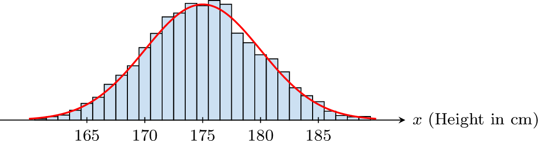
For example, we plot a histogram of the heights of boys at the university. The distribution represented by the histogram follows a bell-shaped curve, also known as a normal distribution.
Definition Standard Normal Distribution
A continuous random variable \(X\) follows a standard normal distribution if it has a mean of 0 and a variance of 1. Its density is:$$f(x) = \frac{1}{\sqrt{2\pi}} e^{-\frac{x^2}{2}}, \quad -\infty < x < \infty$$This is denoted \(X \sim \mathcal{N}(0, 1)\).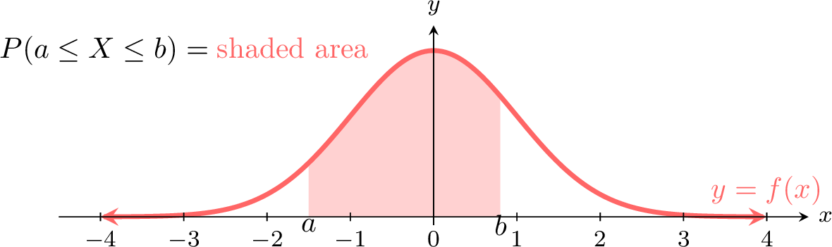
Remark
The total probability is 1:$$\int_{-\infty}^{\infty} \frac{1}{\sqrt{2\pi}} e^{-\frac{x^2}{2}} \, dx = 1$$This is the area under the entire curve.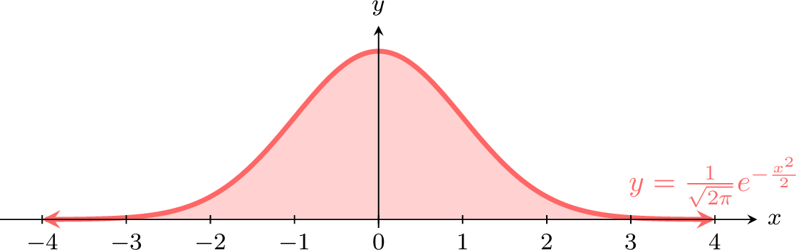
Normal Distribution
Definition Normal Distribution
A continuous random variable \(X\) follows a normal distribution if its density is:$$f(x) = \frac{1}{\sigma \sqrt{2\pi}} e^{-\frac{1}{2} \left( \frac{x - \mu}{\sigma} \right)^2}, \quad -\infty < x < \infty$$where \(\mu\) is the mean and \(\sigma^2\) is the variance. The graph is a normal curve (bell-shaped), denoted \(X \sim \mathcal{N}(\mu, \sigma^2)\).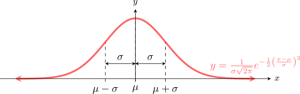
Note on Technology Use
The integral of the normal distribution's probability density function cannot be expressed in terms of elementary functions. Therefore, calculating probabilities for a normal distribution, such as \(P(a \leq X \leq b)\), must be done using a graphic display calculator (GDC) or statistical software.
Proposition Expectation and Variance
For \(X \sim \mathcal{N}(\mu, \sigma^2)\):
- \(E(X) = \mu\),
- \(V(X) = \sigma^2\).
Empirical Rule for Normal Distribution
Proposition Empirical Rule for Normal Distribution
For \(X \sim \mathcal{N}(\mu, \sigma^2)\), the probabilities for intervals centered at the mean are approximately: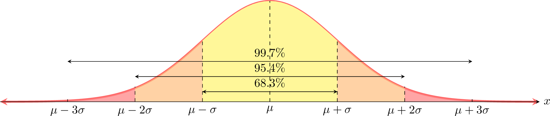
- \(P(\mu - \sigma \leq X \leq \mu + \sigma) \approx 68.3\pourcent\)
- \(P(\mu - 2\sigma \leq X \leq \mu + 2\sigma) \approx 95.4\pourcent\)
- \(P(\mu - 3\sigma \leq X \leq \mu + 3\sigma) \approx 99.7\pourcent\)
The Empirical Rule states that for a normal distribution, specific percentages of data lie within intervals around the mean. Due to the symmetry of the normal curve, we can break these down to find the probabilities for individual sections, each one standard deviation wide. For example, by symmetry, the area from \(\mu\) to \(\mu+\sigma\) is half of the total area from \(\mu-\sigma\) to \(\mu+\sigma\): $$P(\mu \leq X \leq \mu + \sigma) = \frac{P(\mu - \sigma \leq X \leq \mu + \sigma)}{2} \approx 34.13\pourcent$$This gives us a detailed map of the normal distribution: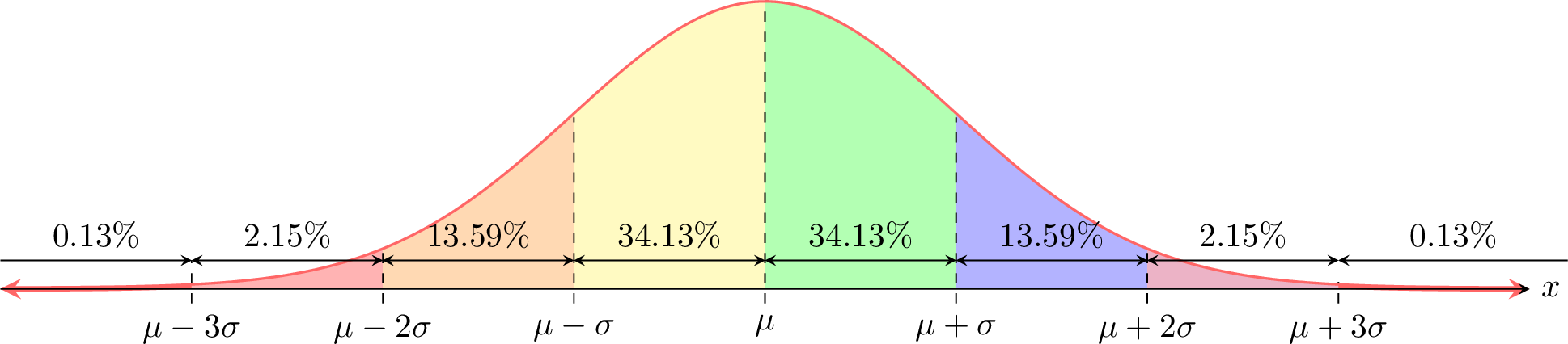
Example
Students’ heights at a school are normally distributed with mean \(\mu = 172 \, \text{cm}\) and standard deviation \(\sigma = 8 \, \text{cm}\).
- Find the percentage of students with heights between 164 cm and 172 cm.
- Find the percentage between 164 cm and 180 cm.
- Find the percentage with heights above 196 cm.
- Find the percentage with heights below 196 cm.
- In a group of 500 students, how many are expected to have heights between 164 cm and 180 cm?
First, we label the distribution with the given mean and standard deviation: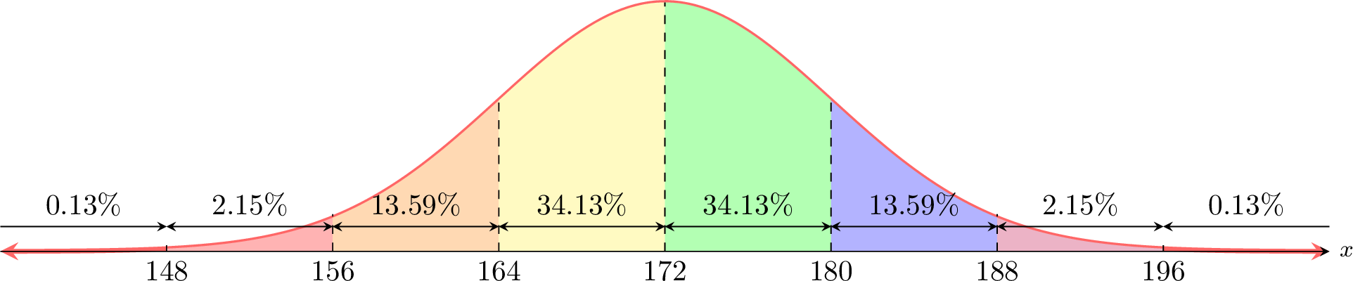
- \(P(164 \leq X \leq 172) = P(\mu - \sigma \leq X \leq \mu) = 34.13\pourcent\).
- \(P(164 \leq X \leq 180) = P(\mu - \sigma \leq X \leq \mu + \sigma) = 34.13\pourcent + 34.13\pourcent = 68.26\pourcent\).
- \(P(X > 196) = P(X \geq \mu + 3\sigma) = 0.13\pourcent\).
- \(P(X < 196) = 1 - P(X \geq 196) = 100\pourcent - 0.13\pourcent = 99.87\pourcent\).
- Expected number = \(68.26\pourcent \times 500 = 0.6826 \times 500 \approx 341\) students.
Quantiles
Definition Quantile
The \(p\)-quantile of a random variable \(X\) is the value \(x_p\) such that \(P(X \leq x_p) = p\). For example, the \(0.95\)-quantile (or 95th percentile) is the value \(x_{0.95}\) below which 95\(\pourcent\) of the distribution's values lie.
Example
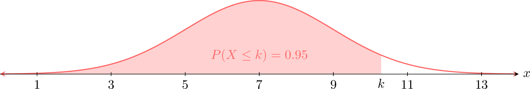
Let \(X \sim \mathcal{N}(7, 2^2)\). Find the value \(k\) such that \(P(X \leq k) = 0.95\).
Using a calculator's inverse normal function with area\(=0.95\), \(\mu = 7\), and \(\sigma = 2\), we find \(k \approx 10.29\).