Coupled Differential Equations

In the previous chapter, we studied single differential equations describing a single quantity changing over time. However, in the real world, systems often involve multiple variables that interact with one another. For example, the population of predators (like foxes) depends on the population of prey (like rabbits), and vice versa.
These situations are modeled by coupled differential equations. In this chapter, we will learn how to visualize these systems using phase portraits, solve systems of linear equations using matrices, eigenvalues, and eigenvectors, and approximate solutions using Euler's method.

A system of coupled first-order differential equations usually takes the form:$$\begin{cases}\dfrac{dx}{dt} = f(x, y) \\ \dfrac{dy}{dt} = g(x, y)\end{cases}$$Here, \(t\) is the independent variable (often time), while \(x\) and \(y\) are the dependent variables (state variables).
We often denote the time derivatives using dot notation: \(\dot{x} = \dfrac{dx}{dt}\) and \(\dot{y} = \dfrac{dy}{dt}\).

An equilibrium point is a state where the system does not change. This occurs when both derivatives are zero simultaneously:$$ \frac{dx}{dt} = 0 \quad \text{and} \quad \frac{dy}{dt} = 0 $$

Consider the system:$$ \frac{dx}{dt} = y \quad \text{and} \quad \frac{dy}{dt} = -x $$To find the equilibrium points, we set both derivatives to zero:$$ y = 0 \quad \text{and} \quad -x = 0 $$The only solution is \((x, y) = (0, 0)\). Thus, the origin is the only equilibrium point.

A phase portrait is a graphical representation where:

• The axes represent the state variables \(x\) and \(y\) (not \(t\)).
• At each point \((x, y)\), the vector \(\begin{pmatrix} \dot{x} \\ \dot{y} \end{pmatrix}\) indicates the direction and speed of change.
• Trajectories are curves that follow the flow of these vectors, showing how the state of the system evolves over time starting from a specific initial condition.

Consider the system:$$ \frac{dx}{dt} = y \quad \text{and} \quad \frac{dy}{dt} = -x $$Let's calculate the velocity vector at a few points: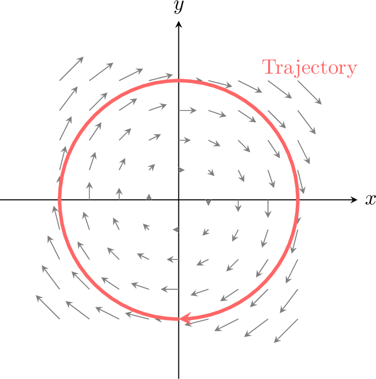

• At \((1, 0)\), vector is \(\begin{pmatrix} 0 \\ -1 \end{pmatrix}\) (Straight down).
• At \((0, -1)\), vector is \(\begin{pmatrix} -1 \\ 0 \end{pmatrix}\) (Straight left).
• At \((-1, 0)\), vector is \(\begin{pmatrix} 0 \\ 1 \end{pmatrix}\) (Straight up).
• At \((0, 1)\), vector is \(\begin{pmatrix} 1 \\ 0 \end{pmatrix}\) (Straight right).

By plotting these, we see the motion is clockwise around the origin.

A fundamental type of coupled system is the linear system with constant coefficients.
These systems can be elegantly solved using matrix algebra. By defining a vector \(\mathbf{x} = \begin{pmatrix} x \\ y \end{pmatrix}\) and a matrix \(\mathbf{A}\), we can condense the system into the compact form \(\dot{\mathbf{x}} = \mathbf{A}\mathbf{x}\).

A system of coupled linear differential equations is a set of equations of the form:$$\begin{cases}\dfrac{dx}{dt} = ax + by \\ \dfrac{dy}{dt} = cx + dy\end{cases}$$This can be written in matrix form as:$$ \begin{pmatrix} \dot{x} \\ \dot{y} \end{pmatrix} = \begin{pmatrix} a & b \\ c & d \end{pmatrix} \begin{pmatrix} x \\ y \end{pmatrix} \iff \dot{\mathbf{x}} = \mathbf{A}\mathbf{x} $$where \(\mathbf{A} = \begin{pmatrix} a & b \\ c & d \end{pmatrix}\) is the matrix of coefficients.

To find the solution, we look for an analogue to the scalar solution \(x = x_0 e^{kt}\).
If we propose a trial solution of the form \(\mathbf{x} = \mathbf{v}e^{\lambda t}\), differentiating gives \(\dot{\mathbf{x}} = \lambda \mathbf{v}e^{\lambda t}\). Substituting this into the system yields:$$ \lambda \mathbf{v}e^{\lambda t} = \mathbf{A}(\mathbf{v}e^{\lambda t}) \implies \mathbf{A}\mathbf{v} = \lambda \mathbf{v} $$This equation holds true precisely when \(\lambda\) is an eigenvalue of \(\mathbf{A}\) and \(\mathbf{v}\) is the corresponding eigenvector.

Let \(\lambda_1\) and \(\lambda_2\) be the distinct real eigenvalues of matrix \(\mathbf{A}\), with corresponding eigenvectors \(\mathbf{v}_1\) and \(\mathbf{v}_2\). The general solution is:$$ \mathbf{x}(t) = A e^{\lambda_1 t} \mathbf{v}_1 + B e^{\lambda_2 t} \mathbf{v}_2 $$where \(A\) and \(B\) are arbitrary constants determined by initial conditions.

Solve the system \(\begin{cases} \dfrac{dx}{dt} = 4x - 2y \\ \dfrac{dy}{dt} = x + y \end{cases}\).

We can describe the behaviour of the phase portrait around an equilibrium point (after translating it to the origin) based on the eigenvalues \(\lambda_1, \lambda_2\) of the system's matrix.

Stable Node (Sink)	Saddle Point	Unstable Node (Source)
{\small \(\lambda_1, \lambda_2 < 0\)}	{\small \(\lambda_1 > 0 > \lambda_2\)}	{\small \(\lambda_1, \lambda_2 > 0\)}
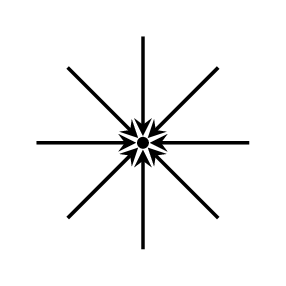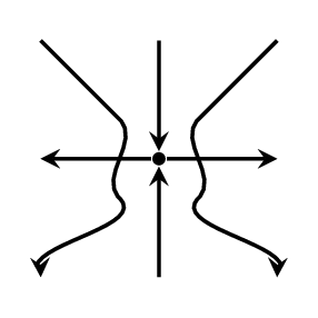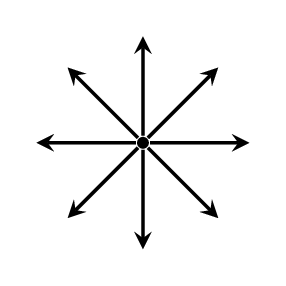Stable Spiral	Center	Unstable Spiral
{\small Complex, Re\((\lambda) < 0\)}	{\small Pure Imaginary}	{\small Complex, Re\((\lambda) > 0\)}

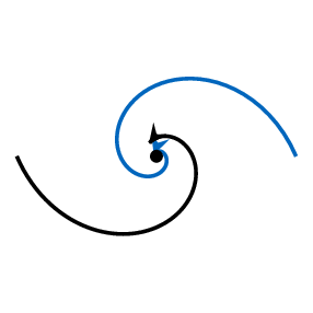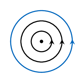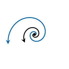Second-order differential equations play a crucial role in physics and engineering. Since Newton's Second Law relates force to acceleration (the second derivative of position), these equations naturally describe mechanical vibrations, such as springs, dampers, and pendulums. Similarly, in electronics, they are essential for modeling the behavior of RLC electrical circuits.

A second-order linear homogeneous differential equation with constant coefficients is an equation of the form:$$ a\frac{d^2x}{dt^2} + b\frac{dx}{dt} + cx = 0 $$where \(a, b,\) and \(c\) are constants and \(a \neq 0\).

• Second-order: The highest derivative is the second derivative.
• Linear: The variable \(x\) and its derivatives appear to the first power and are not multiplied together.
• Homogeneous: The equation equals zero (there is no external forcing term).

Any second-order linear homogeneous differential equation of the form$$ a\frac{d^2x}{dt^2} + b\frac{dx}{dt} + cx = 0 $$can be converted into a system of two first-order equations.

1. Introduce a new variable \(y = \dfrac{dx}{dt}\) (velocity).
2. Differentiate \(y\): \(\dfrac{dy}{dt} = \dfrac{d^2x}{dt^2}\).
3. Rearrange the original equation: \(\dfrac{dy}{dt} = -\frac{b}{a}y - \frac{c}{a}x\).
4. Write as a matrix system: $$ \begin{pmatrix} \dfrac{dx}{dt} \\ \dfrac{dy}{dt} \end{pmatrix} = \begin{pmatrix} 0 & 1 \\ -\frac{c}{a} & -\frac{b}{a} \end{pmatrix} \begin{pmatrix} x \\ y \end{pmatrix} $$

Convert the second-order differential equation \(\dfrac{d^2x}{dt^2} + 3\dfrac{dx}{dt} + 2x = 0\) into a system of coupled first-order equations.

When exact solutions are difficult to find (e.g., non-linear systems), we use Euler's method to approximate the trajectory. For a system \(\dfrac{dx}{dt} = f(x, y)\) and \(\dfrac{dy}{dt} = g(x, y)\) with step size \(h\):

Given initial values \((x_n, y_n)\) at time \(t_n\):

1. Calculate the slopes: \(m_x = f(x_n, y_n)\) and \(m_y = g(x_n, y_n)\).
2. Update the variables: $$ x_{n+1} = x_n + h \cdot m_x $$ $$ y_{n+1} = y_n + h \cdot m_y $$ $$ t_{n+1} = t_n + h $$

Approximate the solution for \(\begin{cases} \dfrac{dx}{dt} = x + y \\ \dfrac{dy}{dt} = x - y \end{cases}\) with initial condition \(x(0)=1, y(0)=0\) and step size \(h=0.1\).