Modelling with Functions
Mathematical modelling is the process of using mathematics to represent, analyse, and predict real-world phenomena. A model typically links measurable variables through a function whose parameters are chosen from data or from reasonable assumptions. From the trajectory of a ball to changes in stock prices, functions provide a precise framework for describing patterns and making informed predictions.
Modelling Cycle
Definition Mathematical Model
A mathematical model is a function (or system of equations) that represents the relationship between variables in a real-world situation.
- The variables represent quantities that can change (e.g., time, height, cost).
- The parameters are constants chosen to fit a context or a data set.
- The model is only intended to be used on a stated domain where it is meaningful.
Example
The relationship between bacterial growth and time can be modelled by the exponential function \(N(t) = N_0e^{kt}\).
Method 5 Steps of Modelling
You should follow these steps:
- Construct: Create a model from data or from a verbal description. This includes choosing a suitable functional form (linear, quadratic, etc.) and determining its parameters.
- Use: Use the model to make predictions.
- Interpolation: Predict within the range of the available data.
- Extrapolation: Predict outside the range of the data (often less reliable).
- Interpret: Explain the meaning of variables and parameters in context (e.g., what does the \(y\)-intercept represent?).
- Evaluate: Assess the validity of the model: compare with data, compute errors, analyse residuals/correlation (if relevant), and check whether the results are realistic.
- Refine: Suggest improvements if the model is inadequate (e.g., ``an exponential model grows too fast; a logistic model may be more appropriate'').
Linear Models
Linear models are the simplest functional models. They describe situations where a quantity changes at a constant rate with respect to another variable. Common applications include cost functions (fixed fee plus hourly rate), distance travelled at constant speed, and currency conversions.
Definition Linear Model
A linear model relates two variables with a constant rate of change:$$ f(x) = mx + c. $$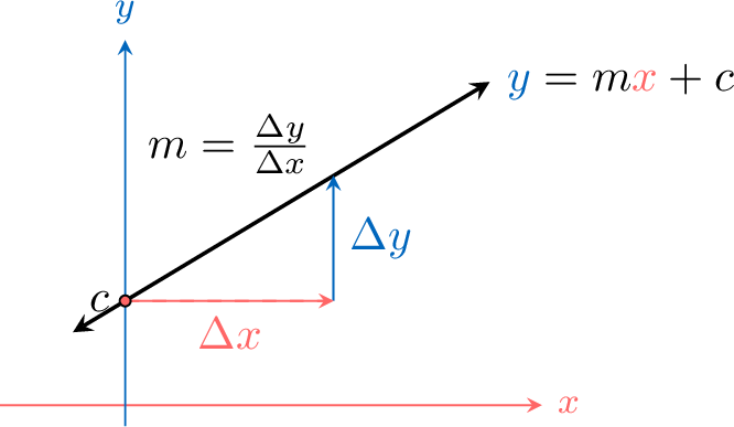
- \(m\): the gradient (rate of change).
- \(c\): the \(y\)-intercept (initial value), i.e. \(f(0)=c\).
Example
A plumber charges a fixed call-out fee of \(\dollar\)50 plus \(\dollar\)80 per hour of work.
The cost model is \(C(t) = 80t + 50\), where \(t\) is the time in hours.
The cost model is \(C(t) = 80t + 50\), where \(t\) is the time in hours.
- Calculate the cost for 10 hours.
- Find the time for the total cost to exceed \(\dollar\)1200.
- Under a new tax, the plumber changes the hourly rate to 80 NZD and the fixed fee to 100 NZD. Write the new cost function after these changes have been made.
- Cost for 10 hours: $$ C(10) = 80(10) + 50 = 800 + 50 = 850. $$ The cost is \(\dollar\)850.
- Time to exceed \(\dollar\)1200: $$ 80t + 50 > 1200 \implies 80t > 1150 \implies t > \frac{1150}{80} = 14.375. $$ So the cost exceeds \(\dollar\)1200 after \(14.375\) hours (i.e.\ 14 hours 22 minutes 30 seconds).
- New cost function: The new hourly rate is 80 NZD and the new fixed fee is 100 NZD: $$ C_{\text{new}}(t) = 80t + 100. $$
Quadratic Models
Quadratic models involve variables raised to the power of 2. They are essential for describing phenomena that have a peak or a valley, such as the path of a projectile under gravity, the area of a rectangle with fixed perimeter, or profit functions in economics.
Definition Quadratic Model
A quadratic model is a function of the form$$ f(x) = ax^2 + bx + c, \qquad a\neq 0. $$
- \(a\) controls the concavity and the vertical stretch/compression.
- \(b\) affects the position of the axis of symmetry.
- \(c\) is the \(y\)-intercept, since \(f(0)=c\).
Proposition Parabola Properties
- If \(a > 0\), the parabola is concave up (opens upwards) and has a minimum value at its vertex:
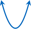 .
. - If \(a < 0\), the parabola is concave down (opens downwards) and has a maximum value at its vertex:
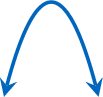 .
.
Example
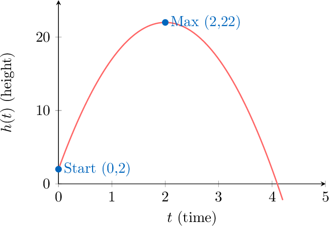
The height of a ball is given by \(h(t) = -5t^2 + 20t + 2\).
- Find the release height.
- Find the maximum height.
- Release height: This is the height at \(t=0\). $$ h(0) = -5(0)^2 + 20(0) + 2 = 2 \text{ m}. $$
- Maximum height: The time of maximum height occurs at the vertex \(t = -\frac{b}{2a}\). Here, \(a=-5\) and \(b=20\), so $$ t = -\frac{20}{2(-5)} = 2 \text{ s}. $$ Now evaluate \(h(2)\): $$ h(2) = -5(2)^2 + 20(2) + 2 = -20 + 40 + 2 = 22 \text{ m}. $$
Cubic Models
Definition Cubic Model
A cubic model is a function of the form$$ f(x)=ax^3+bx^2+cx+d, \qquad a\neq 0. $$
- \(a\) determines the overall end behaviour of the graph and its vertical stretch.
- \(d\) is the \(y\)-intercept, since \(f(0)=d\).
Example
The vertical height of a child above the ground, \(h\) metres, as they go down a water slide can be modelled by the function$$h(t) = \frac{4}{7}(35 - 12t + 6t^2 - t^3),$$where \(t\) is the time in seconds after the child enters the slide.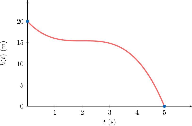
- State the vertical height of the slide.
- Given that the child reaches the ground at the bottom of the slide, find the domain of the function.
- The height of the slide is the initial height at \(t=0\).$$ h(0) = \frac{4}{7}(35) = 20 \text{ m}. $$
- The child reaches the ground when \(h(t) = 0\).$$ \frac{4}{7}(35 - 12t + 6t^2 - t^3) = 0 \implies 35 - 12t + 6t^2 - t^3 = 0. $$Using a calculator or inspection, \(t=5\) is a root:$$ 35 - 12(5) + 6(25) - 125 = 35 - 60 + 150 - 125 = 0. $$Since the child starts at \(t=0\) and reaches the ground at \(t=5\), the physically meaningful domain is \(0 \le t \le 5\).
Exponential Models
Common real-world examples of exponential models include:
- Population growth (growth)
- Radioactive decay (decay)
- Compound interest (growth)
- Cooling of an object (decay)
- Drug concentration in bloodstream (decay)
Definition Exponential Model
An exponential model is a function of the form
- \( f(x) = ka^x + c \), with \( a>0 \) and \( a\neq 1 \)
- \( f(x) = ke^{rx} + c \)
Proposition Properties
- Assume \(k>0\). Exponential growth is represented by:
- \( a^x \) where \( a > 1 \)
- \( e^{rx} \) where \( r > 0 \)
- Assume \(k>0\). Exponential decay is represented by:
- \( a^x \) where \( 0 < a < 1 \)
- \( e^{rx} \) where \( r < 0 \)
- The constant \(c\) translates the graph vertically. When \(r<0\) (or \(0
Example
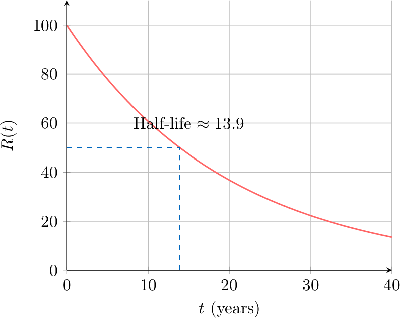
A radioactive element decays according to the formula \(R(t) = 100 e^{-0.05t}\), where \(R\) is the radiation in counts per minute and \(t\) is time in years.
- State the initial radiation.
- Find the half-life (time taken for radiation to halve).
- Initial radiation: At \(t=0\), $$ R(0) = 100 e^0 = 100 \text{ cpm}. $$
- Half-life: We find \(t\) such that \(R(t) = 50\). $$ 50 = 100 e^{-0.05t} \implies 0.5 = e^{-0.05t}. $$ Taking \(\ln\) of both sides: $$ \ln(0.5) = -0.05t \implies t = \frac{\ln(0.5)}{-0.05} \approx 13.86 \text{ years}. $$
Direct/Inverse Variation Models
Variation models describe how one quantity changes in relation to another. They are fundamental in physics and geometry.
Definition Direct Variation
Two variables are said to vary directly if one is a constant multiple of the other.$$ y = kx, \qquad k \text{ constant}. $$Equivalently, for \(x\neq 0\), the ratio \(\frac{y}{x}\) is constant.
Example
- If \( y \) and \( x^n \) (for a positive integer \( n \)) vary directly, then:
- It is denoted as \( y \propto x^n \)
- \( y = kx^n \) for some constant \( k \)
- This can be written as \( \frac{y}{x^n} = k \) (for \(x\neq 0\))
- For \(n \ge 1\), the graph of \(y=kx^n\) passes through the origin \((0,0)\).
Method Find the equation of a direct variation model
- Identify which two variables vary directly (e.g., \(y\) and \(x^2\)).
- Write the generic equation: \(y = kx^n\).
- Use a given pair \((x,y)\) to find the constant \(k\).
- Write the specific equation.
- Use the equation to solve problems.
Example
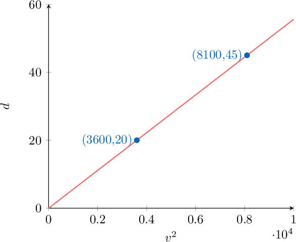
The braking distance, \(d\) metres, of a car varies directly with the square of its speed, \(v\) km/h. A car travelling at 60 km/h has a braking distance of 20 metres.
- Find an equation connecting \(d\) and \(v\).
- Find the braking distance for a car travelling at 90 km/h.
- Equation: We are told \(d \propto v^2\), so \(d = kv^2\). Using \(d=20\) when \(v=60\): $$ 20 = k(60)^2 \implies 20 = 3600k \implies k = \frac{20}{3600} = \frac{1}{180}. $$ Hence \(d = \frac{1}{180}v^2\).
- Prediction: When \(v=90\): $$ d = \frac{1}{180}(90)^2 = \frac{8100}{180} = 45 \text{ metres}. $$
Definition Inverse Variation
Two variables are said to vary inversely if their product is constant:$$ xy = k, \qquad k \text{ constant}. $$Equivalently, for \(x\neq 0\),$$ y = \frac{k}{x}. $$
- This is also called inverse proportion.
Example
If \( y \) and \( x^n \) (for a positive integer \( n \)) vary inversely, then:
- It is denoted as \( y \propto \frac{1}{x^n} \)
- \( y = \frac{k}{x^n} \) for some constant \( k \)
- This can be written as \( yx^n = k \)
Proposition Asymptotic Behavior
The graphs of inverse variation models have a vertical asymptote at \(x=0\) and, when \(n\ge 1\), a horizontal asymptote at \(y=0\).
Method Find the equation of an inverse variation model
- Identify which two variables vary inversely.
- Write the generic equation: \(y = \frac{k}{x^n}\).
- Use the given information to find the constant \(k\).
- Write the specific equation.
Example
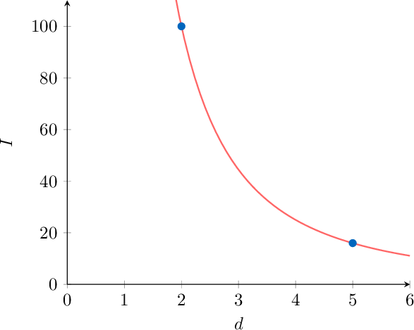
The intensity, \(I\), of light from a bulb varies inversely with the square of the distance, \(d\) metres, from the bulb. At a distance of 2 metres, the intensity is 100 units.
- Write an equation connecting \(I\) and \(d\).
- Find the intensity at a distance of 5 metres.
- Equation: We have \(I \propto \frac{1}{d^2}\), so \(I = \frac{k}{d^2}\). Using \(I=100\) when \(d=2\): $$ 100 = \frac{k}{2^2} \implies 100 = \frac{k}{4} \implies k = 400. $$ Hence \(I = \frac{400}{d^2}\).
- Prediction: When \(d=5\): $$ I = \frac{400}{5^2} = \frac{400}{25} = 16 \text{ units}. $$
Sinusoidal Models
Common real-world examples of sinusoidal models include phenomena that oscillate (fluctuate periodically):
- \(D(t)\) is the depth of water at a shore \(t\) hours after midnight
- \(T(d)\) is the temperature of a city \(d\) days after January 1st
- \(H(t)\) is the vertical height above ground of a person \(t\) seconds after entering a Ferris wheel
Definition Sine and Cosine Models
An Sine/Cosine Model is a function of the form $$y = a\sin(b(x-c)) + d\text{ or }y = a\cos(b(x-c)) + d$$ 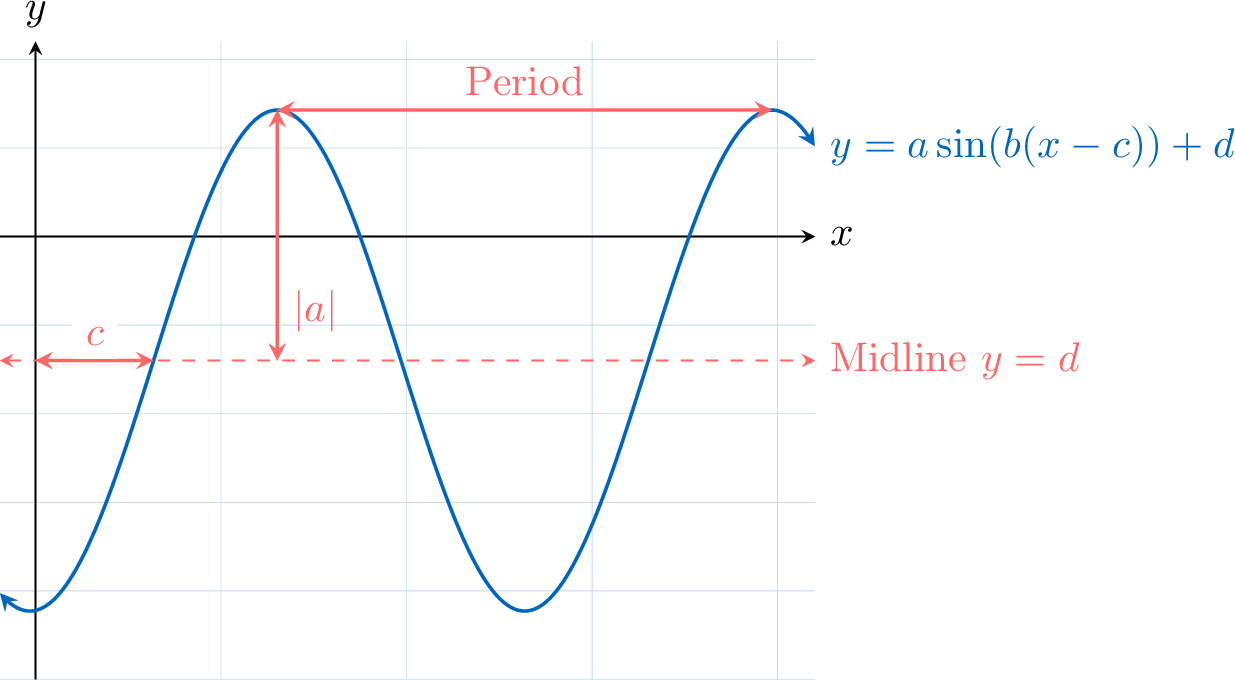
- \(|a|\) is the amplitude.
- \(\frac{2\pi}{|b|}\) (or \(\frac{360}{|b|}\)) is the period.
- \(c\) is the phase shift (horizontal translation).
- \(d\) is the vertical shift (the midline is \(y=d\)).
Example
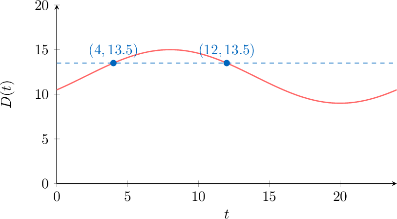
The water depth, \(D\), in metres, at a port can be modelled by the function$$ D(t) = 3 \sin\left( \frac{\pi}{12} (t - 2) \right) + 12, \quad 0 \leq t < 24 $$where \(t\) is the elapsed time, in hours, since midnight.
- Write down the depth of the water at midnight.
- Find the minimum water depth and the time it occurs.
- Calculate how long the water depth is at least 13.5 metres each day.
- At midnight (\(t=0\)): $$ D(0) = 3 \sin\left( \frac{\pi}{12} (0 - 2) \right) + 12 = 3 \sin\!\left(-\frac{\pi}{6}\right) + 12. $$ $$ D(0) = 3(-0.5) + 12 = 10.5 \text{ metres}. $$
- Minimum depth: The sine function ranges from \(-1\) to \(1\), so the minimum occurs when \(\sin(\dots)=-1\): $$ D_{\min} = 3(-1) + 12 = 9 \text{ metres}. $$ This occurs when the argument equals \(-\frac{\pi}{2} + 2\pi k\). In the interval \(0\le t<24\), we may use \(\frac{3\pi}{2}\): $$ \frac{\pi}{12}(t-2) = \frac{3\pi}{2} \implies t-2 = 18 \implies t = 20 \text{ hours (8 PM)}. $$
- Depth \(\ge 13.5\): $$ 3 \sin\left( \frac{\pi}{12} (t - 2) \right) + 12 \ge 13.5 \iff \sin\left( \frac{\pi}{12} (t - 2) \right) \ge 0.5. $$ The equality \(\sin\theta=0.5\) occurs at \(\theta=\frac{\pi}{6}\) and \(\theta=\frac{5\pi}{6}\) (within one period).
- \(\frac{\pi}{12}(t-2) = \frac{\pi}{6} \implies t-2 = 2 \implies t=4\).
- \(\frac{\pi}{12}(t-2) = \frac{5\pi}{6} \implies t-2 = 10 \implies t=12\).
Logarithmic Models
Logarithmic models are often used to measure magnitude or intensity. Common real-world examples include:
- \(M(I)\): the magnitude of an earthquake with an intensity of \(I\) (Richter scale).
- \(d(I)\): the loudness in decibels of a noise with an intensity of \(I\).
- \(\text{pH}(H^+)\): the acidity of a solution based on hydrogen ion concentration.
Definition Logarithmic Model
A logarithmic model is a function of the form$$ f(x) = a + b\ln x, \qquad x>0,\; b\neq 0. $$
- \(\ln x\) denotes the natural logarithm (base \(e\)).
- \(a\) is the value of the function at \(x=1\), since \(f(1)=a\).
- \(b\) controls the rate of increase/decrease.
Proposition Properties
- The graph has a vertical asymptote at the \(y\)-axis (\(x=0\)).
- The function has one root (an \(x\)-intercept) given by $$ f(x)=0 \iff x=e^{-\frac{a}{b}}. $$
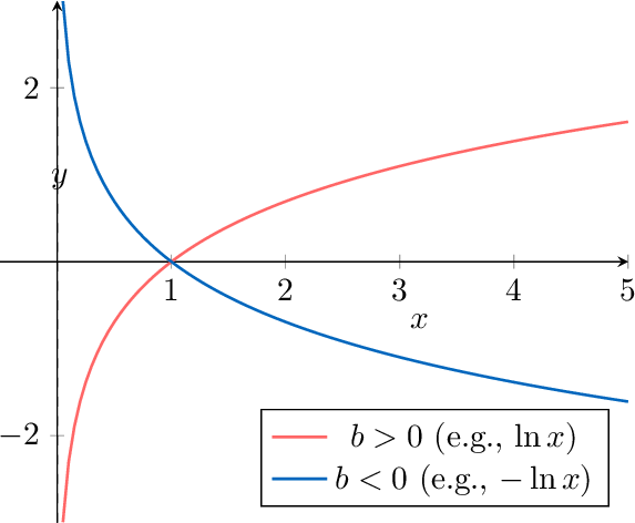
- If \(b > 0\), the function is increasing on \((0,+\infty)\). If \(b < 0\), the function is decreasing on \((0,+\infty)\).
Example
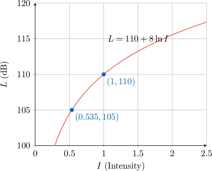
The sound intensity level, \(L\), in decibels (dB) can be modelled by the function$$ L(I) = a + 8 \ln I $$where \(I\) is the sound intensity, in watts per square metre (Wm\(^{-2}\)).
- Given that a sound intensity of \(1 \text{ Wm}^{-2}\) produces a sound intensity level of \(110 \text{ dB}\), write down the value of \(a\).
- Find the sound intensity, in Wm\(^{-2}\), of a car alarm that has a sound intensity level of \(105 \text{ dB}\).
- Find \(a\): Substitute \(I=1\) and \(L=110\): $$ 110 = a + 8 \ln(1). $$ Since \(\ln(1)=0\): $$ a = 110. $$ So, \(L(I) = 110 + 8 \ln I\).
- Find \(I\) when \(L=105\): $$ 105 = 110 + 8 \ln I \implies -5 = 8 \ln I \implies \ln I = -\frac{5}{8}. $$ Therefore, $$ I = e^{-5/8} \approx 0.535 \text{ Wm}^{-2}. $$
Logistic Models
A logistic model is used when a variable initially increases rapidly but then slows down as it approaches a limiting value (saturation). Examples include:
- \(H(t)\): the height of a giraffe \(t\) weeks after birth.
- \(P(t)\): the population of rabbits in a woodland area with limited food.
- The spread of a rumour or a virus in a fixed population.
Definition Logistic Model
A logistic model is of the form$$ f(x) = \frac{L}{1 + Ce^{-kx}}, \qquad L>0,\; k>0. $$
- \(L\) is the carrying capacity (limiting value). It is the horizontal asymptote \(y=L\) as \(x \to +\infty\).
- \(C\) determines the initial value: \(f(0)=\frac{L}{1+C}\) (assuming \(1+C\neq 0\)).
- \(k\) determines the rate of growth.
Example
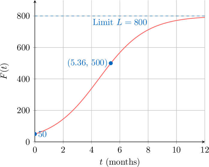
The number of fish in a lake, \(F\), can be modelled by the function$$ F(t) = \frac{800}{1 + Ce^{-0.6t}} $$where \(t\) is the number of months after fish were introduced to the lake.
- Initially, 50 fish were introduced to the lake. Find the value of \(C\).
- Write down the limiting capacity for the number of fish in the lake.
- Calculate the number of months it takes until there are 500 fish in the lake.
- Find \(C\): At \(t=0\), \(F=50\). $$ 50 = \frac{800}{1 + Ce^0} = \frac{800}{1+C}. $$ Hence $$ 1 + C = \frac{800}{50} = 16 \implies C = 15. $$ So, \(F(t) = \frac{800}{1 + 15e^{-0.6t}}\).
- Limiting capacity: $$ L = 800 \text{ fish}. $$
- Find \(t\) when \(F=500\): $$ 500 = \frac{800}{1 + 15e^{-0.6t}} \implies 1 + 15e^{-0.6t} = \frac{800}{500} = 1.6. $$ $$ 15e^{-0.6t} = 0.6 \implies e^{-0.6t} = 0.04. $$ $$ -0.6t = \ln(0.04) \implies t = \frac{\ln(0.04)}{-0.6} \approx 5.36 \text{ months}. $$
Piecewise Linear Models
Piecewise linear models are used when the rate of change of a function differs across intervals. These commonly apply to tariffs, tax brackets, or physical motion.
Definition Piecewise Linear Model
A piecewise linear model is defined by different linear rules on different parts of the domain:$$ f(x) = \begin{cases}m_1x + c_1 & \text{if } x \le a,\\
m_2x + c_2 & \text{if } x > a.\end{cases} $$
- The model may be continuous or discontinuous at the change point \(x=a\).
- If it is continuous and the gradient changes, the graph has a ``corner'' (a kink) at \(x=a\).
Example
The total monthly charge, \(\dollar C\), of a phone bill can be modelled by the function:$$C(m) = \begin{cases}10 + 0.02m & 0 \leq m \leq 100 \\
9 + 0.03m & m > 100\end{cases}$$where \(m\) is the number of minutes used.
- Find the total monthly charge if 80 minutes have been used.
- Given that the total monthly charge is \(\dollar\)16.59, find the number of minutes that were used.
- Calculate cost for \(m=80\): Since \(80 \le 100\), use the first rule: $$ C(80) = 10 + 0.02(80) = 10 + 1.60 = 11.60\dollar. $$
- Calculate minutes for \(C=16.59\): First compute the cost at the end of the first interval: $$ C(100) = 10 + 0.02(100) = 12. $$ Since \(16.59 > 12\), we must have \(m>100\), so use the second rule: $$\begin{aligned} 16.59 &= 9 + 0.03m \\ 7.59 &= 0.03m \\ m &= \frac{7.59}{0.03}\\ m&= 253. \end{aligned} $$ Therefore, \(m=253\) minutes.
