Integrals

The measurement of area has been fundamental to science and society since antiquity. In ancient Egypt, surveyors used knotted ropes to construct right angles, allowing them to measure and restore the boundaries of rectangular fields washed away by the annual floods of the Nile. While finding the area of shapes with straight sides is straightforward, calculus provides a revolutionary tool for finding the area of regions bounded by curves.

In this chapter, we will develop a method to find the exact area, $\mathcal{A}$, of the region bounded by the graph of a function $y=f(x)$, the x-axis, and the vertical lines $x=a$ and $x=b$. This area is denoted by the definite integral:

Approximating Area with Riemann Sums

Method Approximating Area with Riemann Sums

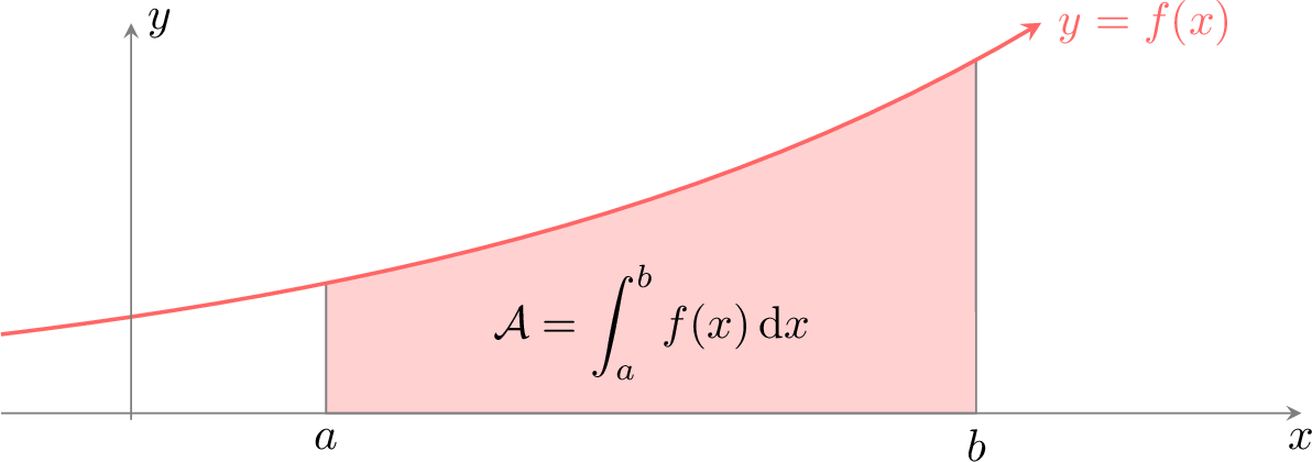
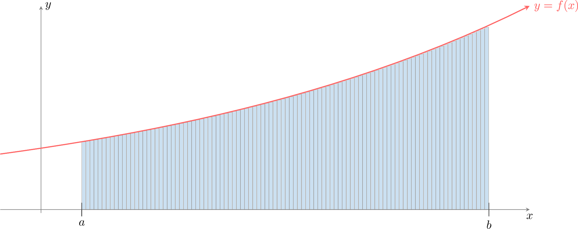
We aim to measure the shaded area, denoted $\displaystyle\int_a^b f(x)\,\mathrm dx$, under the curve of a non-negative function $y=f(x)$.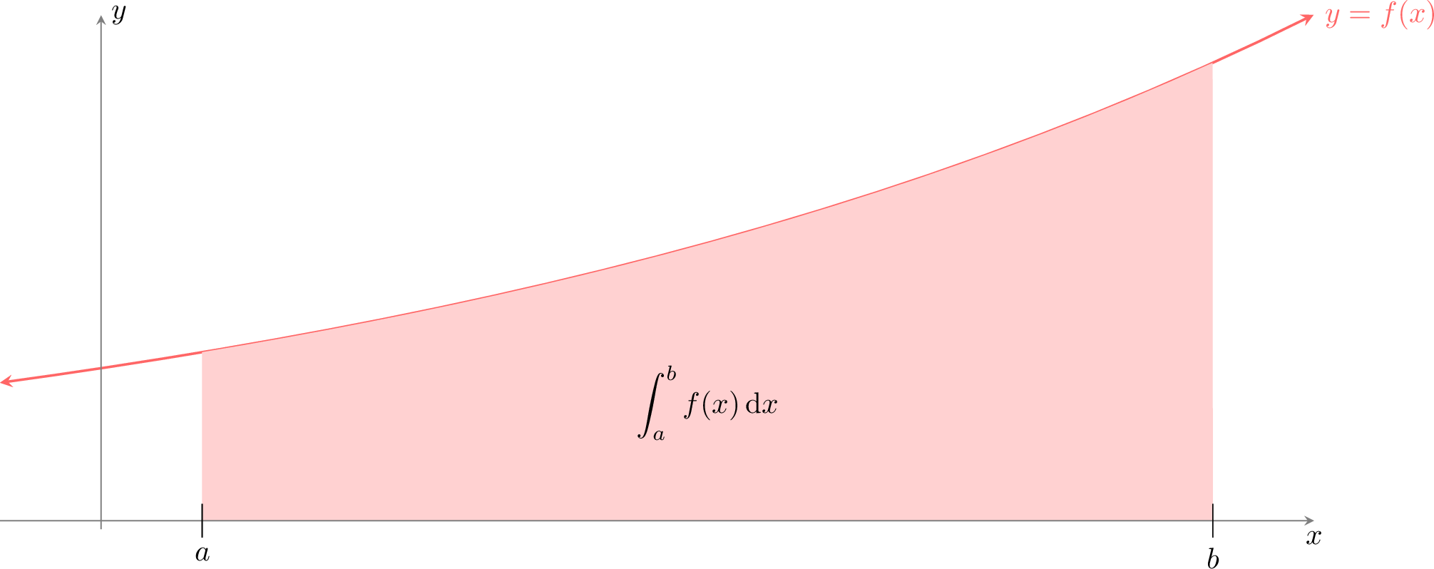

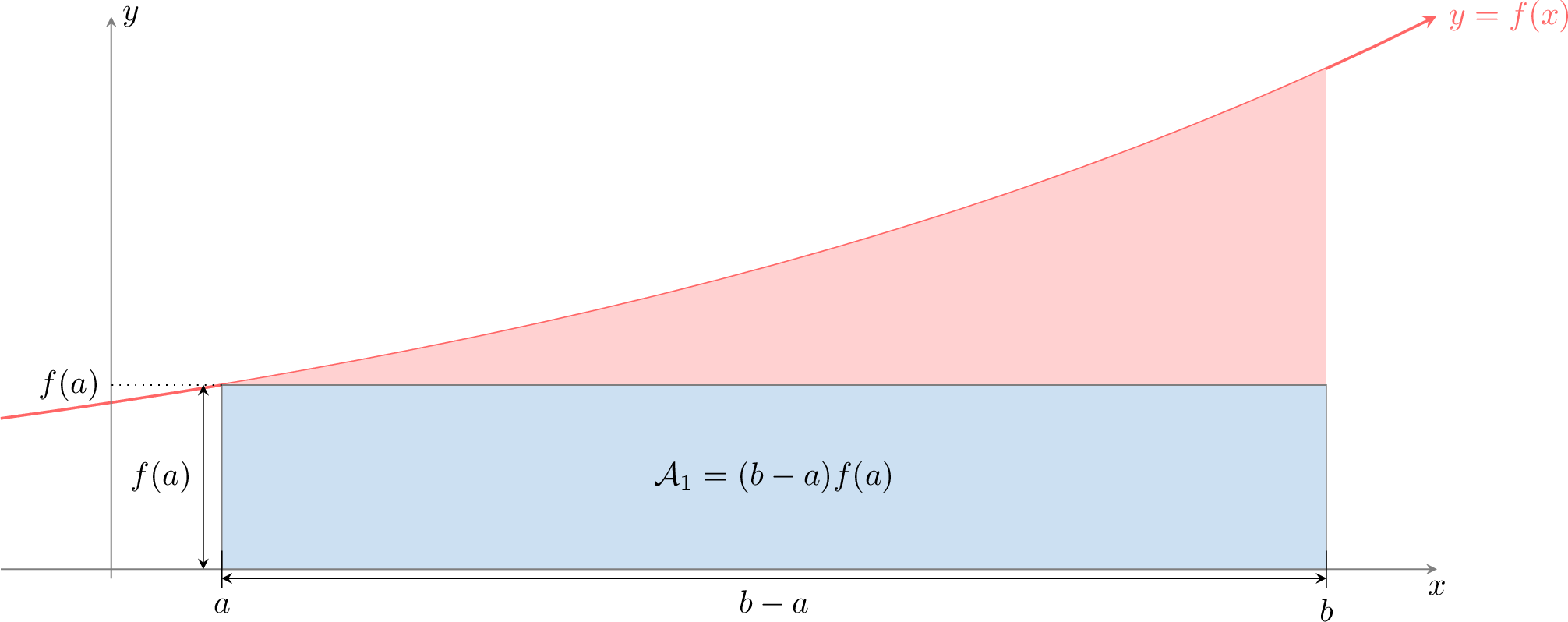
The key idea, developed by Bernhard Riemann, is to approximate this area by a sum of thin rectangles, known as a Riemann sum.

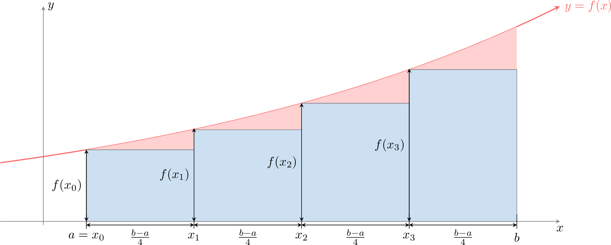
Approximation with 1 rectangle: We can make a first, rough approximation by filling the area with a single rectangle of width $(b-a)$ and height $f(a)$ (the value of the function at the left endpoint).The area is approximated by:$$\displaystyle\int_a^b f(x)\,\mathrm dx \approx (b-a)f(a)$$This is clearly an underestimation.
Approximation with 4 rectangles: To improve the approximation, we divide the interval $[a,b]$ into 4 equal subintervals, each of width $\frac{b-a}{4}$. We construct a rectangle on each subinterval, using the function's value at the left endpoint for the height.The total area of these four rectangles gives a much better approximation:$$\begin{aligned}[t]\displaystyle\int_a^b f(x)\,\mathrm dx &\approx \frac{b-a}{4}f(x_0)+\frac{b-a}{4}f(x_1)+\frac{b-a}{4}f(x_2)+\frac{b-a}{4}f(x_3) \\ &\approx \frac{b-a}{4} \left[f(x_0)+f(x_1)+f(x_2)+f(x_3)\right]\end{aligned}$$
Approximation with $n$ rectangles: We can generalize this by dividing the interval into $n$ equal subintervals, each of width $\Delta x = \frac{b-a}{n}$. Let $x_i=a+i\Delta x$ for $i=0,1,\dots,n-1$. The sum of the areas of the $n$ rectangles is:$$ S_n = \sum_{i=0}^{n-1} f(x_i) \Delta x. $$As we increase the number of rectangles ($n \to \infty$), the width of each rectangle becomes infinitesimally small, and the sum of their areas becomes a perfect match for the area under the curve:$$\displaystyle\int_a^b f(x)\,\mathrm dx = \lim_{n\to\infty} S_n.$$

Definition of the Definite Integral

Definition Definite Integral

The definite integral of a continuous function $f$ from $a$ to $b$ is the limit of the Riemann sum as the number of subintervals approaches infinity. It is denoted by:$$ \int_a^b f(x)\,\mathrm dx = \lim_{n \to \infty} \sum_{i=0}^{n-1} f(x_i) \Delta x $$where the interval $[a,b]$ is divided into $n$ subintervals of equal width $\Delta x = \dfrac{b-a}{n}$ and $x_i$ is a sample point in the $i$th subinterval.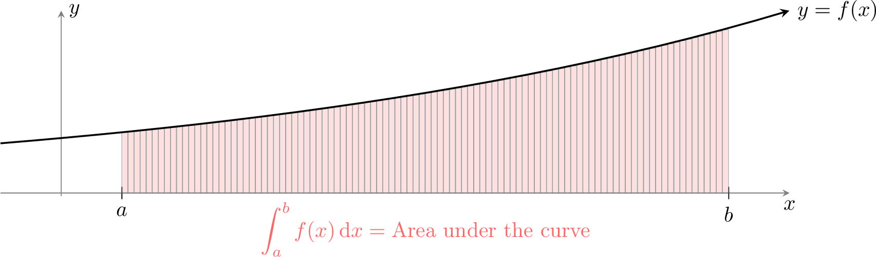

$a$ and $b$ are the limits of integration.
$f(x)$ is the integrand.

This notation, introduced by Leibniz, captures the idea of summing ($ \int $ is an elongated 'S' for summa) the areas of infinitely many rectangles of height $f(x)$ and infinitesimal width $dx$.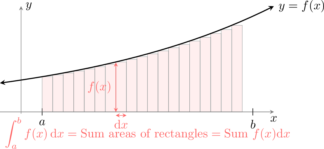

Definition Signed Area

The definite integral calculates the signed area.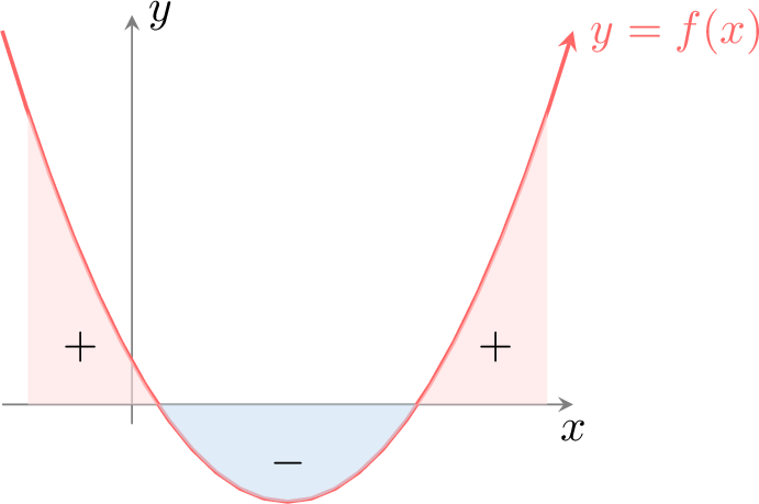

Area above the x-axis is counted as positive.
Area below the x-axis is counted as negative.

The integral is the sum of these signed areas.

Example

Determine the integral $\displaystyle\int_{-1}^{2} 1\,\mathrm dx$ by interpreting it as an area.

Answer

The integral represents the area under the constant function $f(x)=1$ from $x=-1$ to $x=2$. This forms a rectangle with width $2 - (-1) = 3$ and height $1$.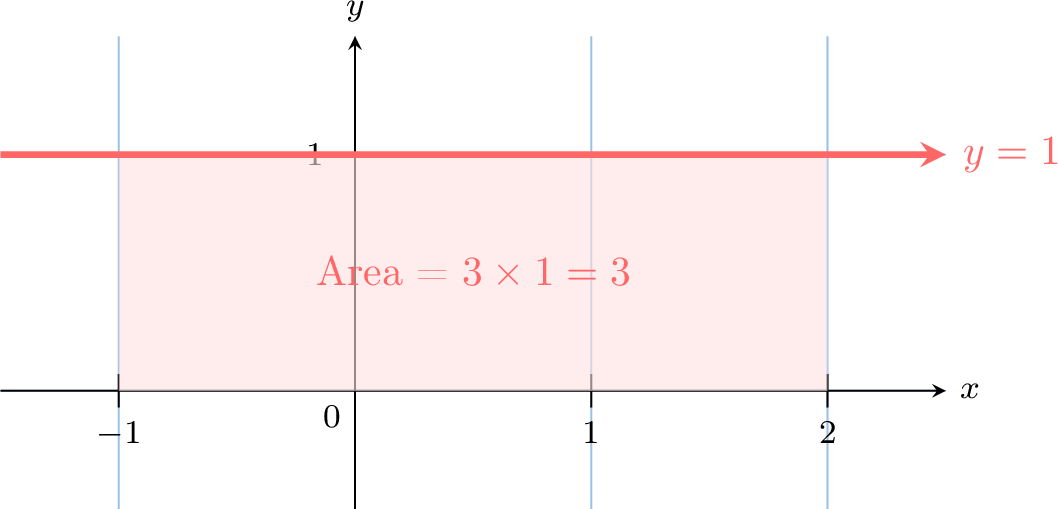

Therefore, $\displaystyle\int_{-1}^{2}1\,\mathrm dx= 3.$

Properties of the Definite Integral

Proposition Properties of Integration

Let $f$ and $g$ be continuous functions and $k$ be a constant.

Zero-Width Interval:$$\displaystyle\int_a^a f(x) \;dx= 0.$$
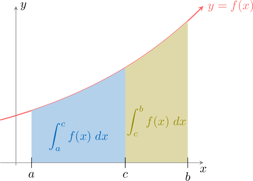
Additivity of Intervals (Chasles's Relation): For any $c$ between $a$ and $b$:$$\displaystyle\int_a^b f(x)\;dx = \int_a^c f(x) \; dx + \int_c^b f(x)\;dx$$
Linearity:$$\displaystyle\int_a^b (f(x)+g(x)) \; dx= \int_a^b f(x) \; dx+ \int_a^b g(x) \; dx$$$$\displaystyle\int_a^b k f(x) \; dx= k \int_a^b f(x) \; dx.$$

Fundamental Theorem of Calculus

So far, we have defined the definite integral as the limit of a sum—a geometric concept of area. Separately, differentiation is a process of finding rates of change. The Fundamental Theorem of Calculus provides a profound and powerful link between these two seemingly unrelated ideas: integration and differentiation are inverse processes of each other.

Theorem Fundamental Theorem of Calculus

If $f$ is a continuous function on the interval $[a,b]$ and $F$ is any antiderivative of $f$, then:$$ \int_a^b f(x)\,\mathrm dx = F(b) - F(a) $$This result is often written using the notation $\left[ F(x) \right]_a^b = F(b)-F(a)$.

Proof

The theorem states that integration and differentiation are inverse processes. We can understand this by examining the "area function".

Defining the Area Function: Let's define a function, $A(x)$, as the area under the curve $y=f(t)$ from a fixed starting point $a$ to a variable endpoint $x$: $$ A(x) = \int_a^x f(t) \, dt. $$ Our goal is to show that the derivative of this area function, $A'(x)$, is simply the original function $f(x)$.
The Area of a Thin Strip: By its definition, the area of a thin vertical strip between $x$ and $x+h$ is the difference between the total area up to $x+h$ and the total area up to $x$: $$ \text{Area of strip} = A(x+h) - A(x). $$
Approximating the Area of the Strip: As shown in the diagram, if the width $h$ is very small, this thin strip is almost a perfect rectangle.
- The width of the rectangle is $h$.
- The height of the rectangle is approximately $f(x)$.
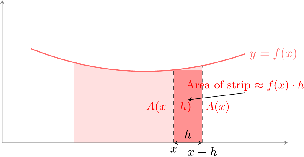
So, we can approximate the strip's area: $$ \text{Area of strip} \approx f(x) \cdot h. $$
Connecting to the Derivative: We now have two expressions for the area of the strip: $$ A(x+h) - A(x) \approx f(x) \cdot h. $$ Dividing both sides by $h$, we get the difference quotient for the function $A(x)$: $$ \frac{A(x+h) - A(x)}{h} \approx f(x). $$
Taking the Limit: This approximation becomes a perfect equality as the width of the strip, $h$, approaches zero. Taking the limit of both sides: $$ \lim_{h\to 0}\frac{A(x+h)-A(x)}{h} = f(x). $$ The expression on the left is, by definition, the derivative of the area function, $A'(x)$: $$ A'(x) = f(x). $$
Finding the Formula: Let $F(x)$ be any antiderivative of $f(x)$. Since all antiderivatives of a function differ only by a constant, we know that: $$ A(x) = F(x) + C $$ for some constant $C$. To find $C$, we can evaluate this at $x=a$: $$ A(a) = \int_a^a f(t)\,dt = 0 $$ so $$ F(a) + C = 0 \implies C = -F(a). $$ Thus the area function is $A(x) = F(x) - F(a)$.
To find the total area up to $x=b$, we simply evaluate $A(b)$: $$ \int_a^b f(x)\,dx = A(b) = F(b) - F(a). $$

Remark

This theorem is fundamental because it connects the geometric concept of area (the definite integral) with the algebraic process of antidifferentiation. It gives us a powerful method to calculate exact areas without using the limit of a Riemann sum.

Example

Find $\displaystyle \int_0^2 x^2 \mathrm dx$.

Answer

Find an antiderivative: An antiderivative of $f(x)=x^2$ is $F(x) = \dfrac{x^3}{3}$.
Apply the Fundamental Theorem: $$\begin{aligned}\displaystyle \int_0^2 x^2 \mathrm dx &= \left[ \frac{x^3}{3} \right]_0^2\\ &= F(2) - F(0) \\ &=\frac{2^3}{3} -\frac{0^3}{3}\\ &=\frac{8}{3} - 0 = \frac{8}{3} \end{aligned}$$

This means the exact area under the curve $y=x^2$ over $[0,2]$ is $\dfrac 8 3$.

Integration by Parts

Integration by parts is a powerful technique for integrating the product of two functions. It is derived from the product rule for differentiation and effectively reverses it.

Proposition Integration by Parts

Let $u$ be differentiable and $v$ be differentiable on $[a, b]$. Then $$ \int_a^b u(x)v'(x) \, dx = \left[u(x)v(x)\right]_a^b - \int_a^b u'(x)v(x) \, dx $$

Proof

The product rule for differentiation states that for two functions $u(x)$ and $v(x)$:$$ \left(u(x)v(x)\right)' = u'(x)v(x) + u(x)v'(x) $$Integrating both sides with respect to $x$:$$ \int \left(u(x)v(x)\right)' \, dx = \int u'(x)v(x) \, dx + \int u(x)v'(x) \, dx $$Since integration is the antiderivative, the left side simplifies to $u(x)v(x)$:$$ u(x)v(x) = \int u'(x)v(x) \, dx + \int u(x)v'(x) \, dx $$Rearranging this equation gives the formula for integration by parts:$$ \int u(x)v'(x) \, dx = u(x)v(x) - \int u'(x)v(x) \, dx $$

Note

The key to using this method is to choose $u$ and $v'$ strategically. The goal is to select a $u$ that becomes simpler when differentiated (e.g., a polynomial) and a $v'$ that is easy to integrate. The new integral, $\int u'v \, dx$, should be easier to solve than the original one.

Example

Find $\displaystyle\int_0^1 x e^x \; dx$.

Answer

We have a product of two functions, $x$ and $e^x$. We choose $u$ and $v'$:

Let $u=x$ (since its derivative $u'=1$ is simpler).
Let $v'=e^x$ (since its antiderivative $v=e^x$ is easy to find).

Now we apply the formula for definite integrals:$$\begin{aligned}\int_0^1 x e^x \; dx & = \left[x e^x\right]_0^1 - \int_0^1 (1) \cdot e^x \;dx \\ & = \left(1\cdot e^1 - 0\cdot e^0\right) - \left[e^x\right]_0^1 \\ & = (e - 0) - (e^1-e^0) \\ & = e - (e-1)\\ & = 1.\end{aligned}$$

Integrals and Inequalities

Proposition Positivity Rule

Let $f$ be a continuous function on an interval $[a, b]$ with $a \le b$.

If $f(x) \ge 0$ for all $x \in [a, b]$, then $\displaystyle \int_{a}^{b} f(x) \,dx \ge 0$.
If $f(x) \le 0$ for all $x \in [a, b]$, then $\displaystyle \int_{a}^{b} f(x) \,dx \le 0$.

Proposition Comparison Rule

Let $f$ and $g$ be two continuous functions on $[a, b]$ with $a \le b$.
If $f(x) \le g(x)$ for all $x \in [a, b]$, then:$$ \int_{a}^{b} f(x) \,dx \le \int_{a}^{b} g(x) \,dx $$

Proof

If $f(x) \le g(x)$, then $g(x) - f(x) \ge 0$.
By the Positivity Rule, $\displaystyle \int_{a}^{b} (g(x) - f(x)) \,dx \ge 0$.
Using the Linearity Property:$$ \int_{a}^{b} g(x) \,dx - \int_{a}^{b} f(x) \,dx \ge 0 \implies \int_{a}^{b} f(x) \,dx \le \int_{a}^{b} g(x) \,dx $$

Definition Mean Value

The mean value of a continuous function $f$ on an interval $[a, b]$ (where $a \neq b$) is the real number $\mu$ defined by:$$ \mu = \frac{1}{b - a} \int_{a}^{b} f(x) \,dx $$

Graphical Interpretation

In the case where $f$ is positive on $[a, b]$, the equality $\displaystyle \int_{a}^{b} f(x) \,dx = \mu(b - a)$ indicates that the area of the domain under the graph of $f$ is equal to the area of the rectangle with dimensions $\mu$ and $b - a$.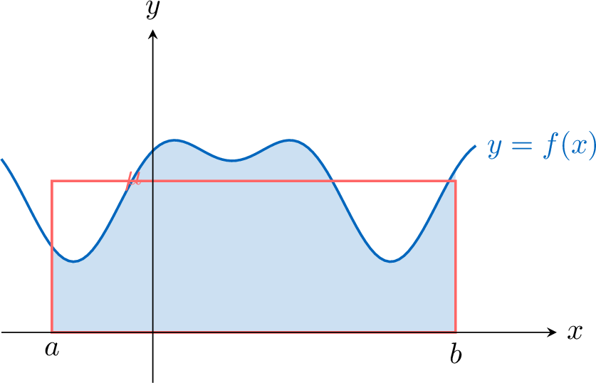

Area Between Two Curves

We can extend the concept of finding the area under a single curve to find the area of a region enclosed between two different curves. The area under a curve $y=f(x)$ is a special case where the second curve is simply the $x$-axis, $y=0$.
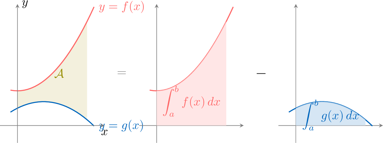
The general idea is intuitive: the area of the region bounded by an upper function $f(x)$ and a lower function $g(x)$ is found by calculating the area under $f(x)$ and subtracting the area under $g(x)$. Using the linearity of the definite integral, this subtraction can be combined into a single integral:$$\begin{aligned} \textcolor{olive}{\mathcal{A}} &= \textcolor{colordef}{ \int_a^b f(x)\; \mathrm dx} - \textcolor{colorprop}{ \int_a^b g(x)\; \mathrm dx} \\ &= \int_a^b (f(x)-g(x))\; \mathrm dx \end{aligned} $$

Proposition Area Between Curves

If $f(x) \geq g(x)$ for all $x$ in the interval $[a,b]$, the area $\mathcal{A}$ of the region enclosed between the curves $y=f(x)$ and $y=g(x)$ is given by:$$ \mathcal{A} = \int_a^b (f(x)-g(x))\; \mathrm dx $$

This can be remembered as the integral of the upper function minus the lower function.

Method Calculating the Area Between Two Curves

To find the total geometric area enclosed by two curves $y=f(x)$ and $y=g(x)$:

Find points of intersection. If the limits of integration $a$ and $b$ are not given, find them by solving the equation $f(x)=g(x)$ to determine where the curves cross.
Identify the upper and lower function. On each interval between intersection points, determine which function is on top. A quick sketch or testing a point is often sufficient.
Set up and evaluate the integral(s). For each interval, calculate $\int_a^b (\text{upper function} - \text{lower function}) \, dx$. If the upper and lower functions switch, you will need to set up multiple integrals and (for geometric area) sum their absolute values.

Example

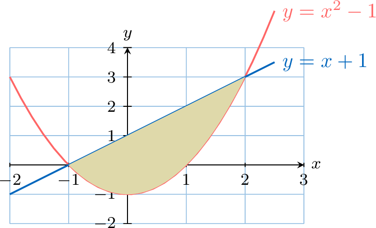
Find the area of the region enclosed by the curves $y=x+1$ and $y=x^2-1$.

Answer

Find intersection points: We set the two functions equal to each other: $$ x+1 = x^2-1 \iff x^2-x-2=0 \iff(x-2)(x+1)=0 $$ The curves intersect at $x=-1$ and $x=2$. These are our limits of integration.
Identify the upper function: In the interval $[-1,2]$, let's test the point $x=0$. For $y=x+1$, $y(0)=1$. For $y=x^2-1$, $y(0)=-1$. Since $1 > -1$, the line $y=x+1$ is the upper function on $[-1,2]$.
Set up and evaluate: $$\begin{aligned} \mathcal{A} &= \int_{-1}^2 \left( (x+1) - (x^2-1) \right)\, dx \\ &= \int_{-1}^2 (-x^2+x+2)\, dx \\ &= \left[ -\frac{x^3}{3} + \frac{x^2}{2} + 2x \right]_{-1}^2 \\ &= \left(-\frac{8}{3} + \frac{4}{2} + 4\right) - \left(\frac{1}{3} + \frac{1}{2} - 2\right) \\ &= \left(-\frac{16}{6} + \frac{12}{6} + \frac{24}{6}\right) - \left(\frac{2}{6} + \frac{3}{6} - \frac{12}{6}\right) \\ &= \frac{20}{6} - \left(\frac{7}{6}\right) \\ &= \frac{27}{6} \\ &= \frac{9}{2} \end{aligned}$$

The area of the enclosed region is $\frac{9}{2}$ square units.