Probability
Ever wondered if it'll rain tomorrow or if you'll win a game? That's probability! It's a math way to guess how likely things are to happen. Like when the weather app says there's a 90\(\pourcent\) chance of rain, that's probability telling us it's very likely. What else do you think we could use probability for?
Algebra of Events
Sample Space
Have you ever flipped a coin and wondered if it’d land on heads or tails? Or rolled a die and guessed what number you’d get? These are random experiments—things we do where the result isn’t certain until it happens.
Definition Outcome
An outcome is one possible result of a random experiment.
Definition Sample Space
The sample space is the list of all possible outcomes of a random experiment.
Example
What’s the sample space when you flip a coin?
It’s \(\{\)Heads, Tails\(\}=\{\) ,
, \(\}\), or just \(\{\)H, T\(\}\) for short.
Example
What’s the sample space when you roll a six-sided die?
It’s \(\{\)1, 2, 3, 4, 5, 6\(\}=\{\) ,
, ,
, ,
, ,
, ,
,  \(\}\).
Events
Definition Event
An event is a set of outcomes from all possible outcomes.
In math, we use capital letters like \(E\) to name events. So, we might say \(E\) is the event “it’s sunny tomorrow.”
Example
You roll a die. Let \(E\) be the event of rolling an even number. What’s \(E\)?
The sample space is \(\{1, 2, 3, 4, 5, 6\}\), and \(E = \{2, 4, 6\}\) because those are the even numbers.
Complementary Event
Definition Complementary Event
The complementary event of an event \(E\) is everything in the sample space that isn’t in \(E\). We call it \(E'\) (\(E\)-prime).
Example
You roll a die, and \(E\) is rolling an even number. What’s \(E'\)?
\(E = \{2, 4, 6\}\), so \(E'\) is all the other numbers: \(E' = \{1, 3, 5\}\). These are the odd numbers!
Multi-Step Random Experiments
A multi-step random experiment is one that involves a sequence of actions, where each action (or step) has its own set of possible outcomes. In our example of tossing two coins, the experiment is multi-step because it involves two separate coin tosses:
- The first coin toss (step 1) can result in Heads (H) or Tails (T).
- The second coin toss (step 2) can also result in Heads (H) or Tails (T).
Method Representations of Multi-Step Random Experiment
When an experiment involves more than one step, we can represent the sample space (the set of all possible outcomes) in several ways:
- using a grid (to visually map combinations along two axes),
- using a table (to organize outcomes in rows and columns),
- using a tree diagram (to follow each sequential step), or
- by listing all possible outcomes.
Example
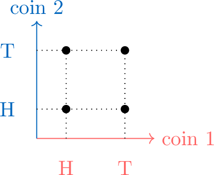
For the random experiment of tossing two coins, display the sample space by:
- using a grid
- using a table
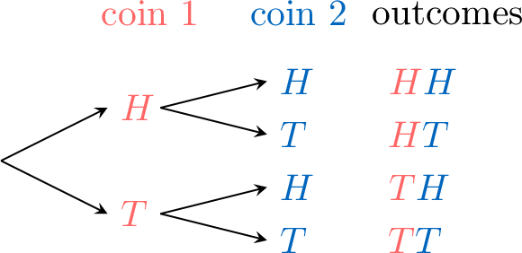
- using a tree diagram
- listing all possible outcomes
-
-
\(\begin{aligned} & \textcolor{colorprop}{\text{coin 2}} \\ \textcolor{colordef}{\text{coin 1}} \end{aligned} \) \(\textcolor{colorprop}{H}\) \(\textcolor{colorprop}{T}\) \(\textcolor{colordef}{H}\) \(\textcolor{colordef}{H}\textcolor{colorprop}{H}\) \(\textcolor{colordef}{H}\textcolor{colorprop}{T}\) \(\textcolor{colordef}{T}\) \(\textcolor{colordef}{T}\textcolor{colorprop}{H}\) \(\textcolor{colordef}{T}\textcolor{colorprop}{T}\) -
- \(\{\textcolor{colordef}{H}\textcolor{colorprop}{H}, \textcolor{colordef}{H}\textcolor{colorprop}{T},\textcolor{colordef}{T}\textcolor{colorprop}{H}, \textcolor{colordef}{T}\textcolor{colorprop}{T}\}\)
\(E\) or \(F\)
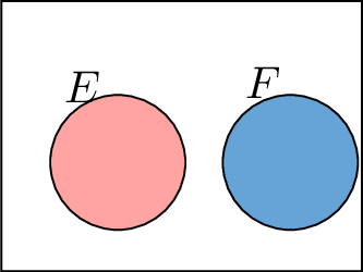
Definition \(E\) or \(F\)
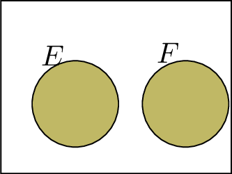
The union of two events \(E\) and \(F\), denoted as \(E \text{ or } F\) or \(E \cup F\), is the event that occurs if either event \(E\) happens, event \(F\) happens, or both events happen simultaneously.
Example
Consider the roll of a standard six-sided die.
Let event \(E\) be the event of rolling an even number. So, \(E = \{2, 4, 6\}\).
Let event \(F\) be the event of rolling a number less than 4. So, \(F = \{1, 2, 3\}\).
Find the event \(E\) or \(F\).
Let event \(E\) be the event of rolling an even number. So, \(E = \{2, 4, 6\}\).
Let event \(F\) be the event of rolling a number less than 4. So, \(F = \{1, 2, 3\}\).
Find the event \(E\) or \(F\).
\(E\) or \(F\) includes all outcomes from both event sets.
So, \(E \text{ or } F = E \cup F = \{1, 2, 3, 4, 6\}\).
So, \(E \text{ or } F = E \cup F = \{1, 2, 3, 4, 6\}\).
\(E\) and \(F\)
Definition \(E\) and \(F\)
$$$$The intersection of two events \(E\) and \(F\), denoted as \(E \text{ and } F\) or \(E \cap F\), is the set of all outcomes that are common to both \(E\) and \(F\). The event \(E\) and \(F\) occurs if and only if both \(E\) and \(F\) happen simultaneously.
Example
Consider the roll of a standard six-sided die.
Let event \(E\) be the event of rolling an odd number. So, \(E = \{1, 3, 5\}\).
Let event \(F\) be the event of rolling a number less than 4. So, \(F = \{1, 2, 3\}\).
Find the event \(E\) and \(F\).
Let event \(E\) be the event of rolling an odd number. So, \(E = \{1, 3, 5\}\).
Let event \(F\) be the event of rolling a number less than 4. So, \(F = \{1, 2, 3\}\).
Find the event \(E\) and \(F\).
\(E\) and \(F\) includes all outcomes that are common to both \(E\) and \(F\).
So, \(E \text{ and } F = E \cap F = \{1, 3\}\).
So, \(E \text{ and } F = E \cap F = \{1, 3\}\).
Mutually Exclusive
Definition Mutually Exclusive
Two events \(E\) and \(F\) are said to be mutually exclusive if they cannot occur simultaneously. In other words, the occurrence of event \(E\) excludes the possibility of event \(F\) occurring, and vice versa. This is mathematically represented as:$$E \text{ and } F = E \cap F = \emptyset,$$where \(\emptyset\) denotes the empty set, indicating that there are no common outcomes between \(E\) and \(F\).
Example
Consider the roll of a standard six-sided die.
Let event \(E\) be the event of rolling an odd number. So, \(E = \{1, 3, 5\}\).
Let event \(F\) be the event of rolling an even number. So, \(F = \{2, 4, 6\}\).
Show that \(E\) and \(F\) are mutually exclusive.
Let event \(E\) be the event of rolling an odd number. So, \(E = \{1, 3, 5\}\).
Let event \(F\) be the event of rolling an even number. So, \(F = \{2, 4, 6\}\).
Show that \(E\) and \(F\) are mutually exclusive.
Since there are no common outcomes between \(E\) and \(F\), we have \(E \text{ and } F = E \cap F = \emptyset\). Thus, the events \(E\) and \(F\) are mutually exclusive.
Venn Diagram
Definition Correspondence Between Set Theory and Probabilistic Vocabulary
| Notation | Set Vocabulary | Probabilistic Vocabulary | Venn Diagram |
| \(U\) | Universal set | Sample space | 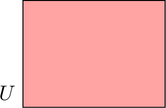 |
| \(x\) | Element of \(U\) | Outcome | 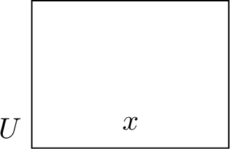 |
| \(\emptyset\) | Empty set | Impossible event | |
| \(E\) | Subset of \(U\) | Event | 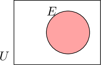 |
| \(x \in E\) | \(x\) is an element of \(E\) | \(x\) is an outcome of \(E\) | 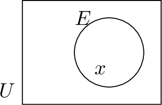 |
| \(E'\) | Complement of \(E\) in \(U\) | Complement of \(E\) in \(U\) | 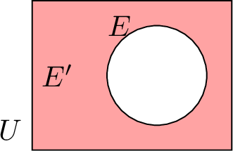 |
| \(E \text{ or } F\) | Union of \(E\) and \(F\): \(E \cup F\) | \(E\) or \(F\) | 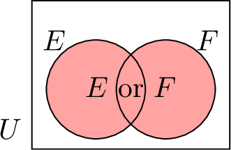 |
| \(E \text{ and } F\) | Intersection of \(E\) and \(F\): \(E \cap F\) | \(E\) and \(F\) | 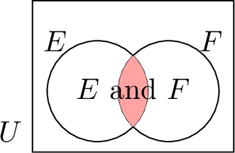 |
| \(E \cap F = \emptyset\) | \(E\) and \(F\) are disjoint | \(E\) and \(F\) are mutually exclusive | 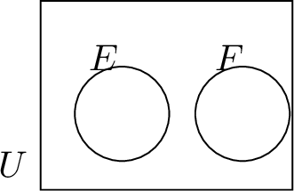 |
Probability
Probability Axioms
The probability of an event \(E\), denoted by \(P(E)\), is a value between 0 and 1 that represents the chance or likelihood of that event occurring.
We can visualize probabilities on a number line: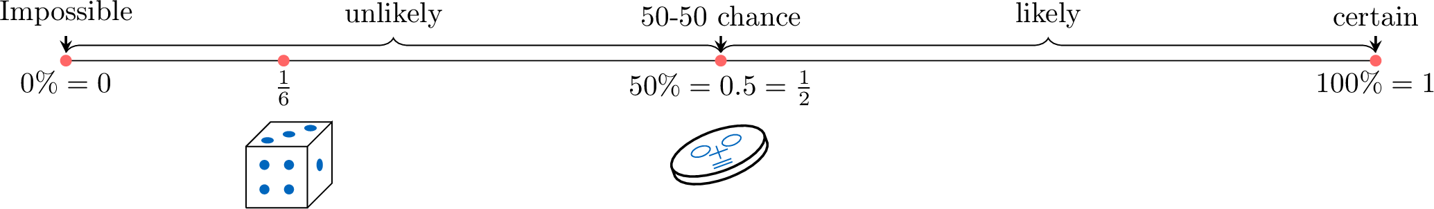
- The probability of an impossible event is \(0\) or \(0\pourcent\).
- The probability of a certain event is \(1\) or \(100\pourcent\).
- The probability of any event is between \(0\) and \(1\), inclusive.
We can visualize probabilities on a number line:
Definition Probability Axioms
\(P\) is a probability if:
- \(0 \leqslant P(E) \leqslant 1\), for any event \(E\),
- \(P(U) = 1\),
- If \(E\) and \(F\) are mutually exclusive events, then \(P(E \text{ or } F) = P(E) + P(F)\).
- The probability of an event \(E\), \(\textcolor{colordef}{P(E)}\), is represented by the shaded area of the event in a Venn diagram:
- The first axiom states that the probability of an event \(E\) is a value between 0 and 1, inclusive.
- The second axiom states that the probability of the sample space \(U\) is equal to \(1\), i.e., \(100\pourcent\). This is because the sample space \(U\) includes all possible outcomes of a random experiment, so the event \(U\) always occurs, and \(P(U) = 1\). In a Venn diagram, this is represented as the entire shaded area of the sample space:$$\textcolor{colordef}{P(U)} = 1$$
- The third axiom states that if two events are mutually exclusive (i.e., they cannot occur simultaneously), then the probability of their union is the sum of their individual probabilities. In a Venn diagram, for two mutually exclusive events (with no overlap), the total area of their union is the sum of the individual areas:
 =
=
Probability Rules
Proposition Complement Rule
For any event \(E\) with complementary event \(E'\),$$\textcolor{colordef}{P(E)} + \textcolor{colorprop}{P(E')} = 1$$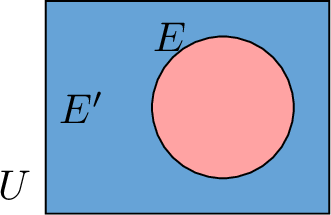
The green area, \(\textcolor{olive}{P(U)}\), ,is the sum of the red area, \(P(E)\), and the blue area, \(P(E')\),
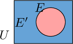 .So,$$\textcolor{colordef}{P(E)} + \textcolor{colorprop}{P(E')} = \textcolor{olive}{P(U)}$$Since \(\textcolor{olive}{P(U) = 1}\), we have:$$\textcolor{colordef}{P(E)} + \textcolor{colorprop}{P(E')} = 1$$
,is the sum of the red area, \(P(E)\), and the blue area, \(P(E')\),.So,$$\textcolor{colordef}{P(E)} + \textcolor{colorprop}{P(E')} = \textcolor{olive}{P(U)}$$Since \(\textcolor{olive}{P(U) = 1}\), we have:$$\textcolor{colordef}{P(E)} + \textcolor{colorprop}{P(E')} = 1$$
Example
Farid has a 0.8 (80\(\pourcent\)) chance of finishing his homework on time tonight (event \(E\)). What’s the chance he doesn’t finish on time ?
The complementary event \(E'\) represents the scenario where Farid does not complete his homework on time tonight. As \(P(E) = 0.8\), by the complement rule, we get:$$\begin{aligned}P(E') &= 1 - 0.8 \\&= 0.2\end{aligned}$$So, there’s a 20 \(\pourcent\) chance he doesn’t finish on time!
Proposition Addition Law of Probability
For any events \(E\) and \(F\),$$P(E \text{ or } F) = P(E) + P(F) - P(E \text{ and } F)$$
Example
A local high school is holding a talent show where students can participate in singing, dancing, or both. The probability that a randomly selected student participates in singing is 0.4, the probability that a student participates in dancing is 0.3, and the probability that a student participates in both singing and dancing is 0.1. Find the probability that a randomly selected student participates in either singing or dancing.
- Let \(S\) be the event that a student participates in singing, and \(D\) be the event that a student participates in dancing. We are given \(P(S) = 0.4\), \(P(D) = 0.3\), and \(P(S \text{ and } D) = 0.1\).
- The probability of either singing or dancing is given by \(P(S \text{ or } D)\).
- By the addition law of probability,$$\begin{aligned}P(S \text{ or } D) &= P(S) + P(D) - P(S \text{ and } D) \\&= 0.4 + 0.3 - 0.1 \\&= 0.6\end{aligned}$$
- Thus, the probability that a student participates in either singing or dancing is \(0.6\).
Equally Likely
Sometimes, every outcome in an experiment has the same chance—like flipping a fair coin or rolling a fair die. We call these equally likely outcomes.
Definition Equally Likely
When all outcomes in a sample space are equally likely, the probability of an event \(E\) within the sample space \(U\) is calculated as:$$\begin{aligned}P(E) &= \frac{\Card{E}}{\Card{U}} \\&= \frac{\text{number of favorable outcomes in the event}}{\text{total number of possible outcomes}}\end{aligned}$$
Example
What’s the probability of rolling an even number with a fair six-sided die?
- Sample space = \(\{1, 2, 3, 4, 5, 6\}\) (6 outcomes).
- \(E = \{2, 4, 6\}\) (3 outcomes).
- $$\begin{aligned}P(E) &= \frac{3}{6}\\&= \frac{1}{2}\end{aligned}$$.
Method Counting Techniques
To calculate the probability of an event, we need to compare the number of favorable outcomes to the total number of possible outcomes in the sample space. But sometimes, listing every single outcome in a sample space would take way too long! That’s where counting techniques come in. Using ideas from chapter on counting, we can figure out the number of outcomes in the sample space without writing them all out one by one.
Example
In a race with 20 horses, you bet on 3 horses to finish first, second, and third in exact order (a "triple forecast"). What’s the probability of winning your bet?
Let’s break it down step by step:
- Total possible outcomes: For a triple forecast, the horses must finish in a specific order.
- You have 20 choices for the horse that finishes 1st.
- After that, 19 horses are left to choose from for 2nd place.
- Then, 18 horses remain for 3rd place.
- So, the total number of possible outcomes in the sample space is: $$ \Card{U} = 20 \times 19 \times 18. $$
- Favorable outcomes: Let \(E\) be the event of correctly predicting one specific triple forecast in order. Since you’re betting on just one exact arrangement of 3 horses (e.g., Horse A first, Horse B second, Horse C third), there’s only 1 way to get it right. Thus: $$ \Card{E} = 1. $$
- Probability calculation: The probability of winning the triple forecast is the ratio of favorable outcomes to total outcomes: $$ \begin{aligned} P(E) &= \frac{\Card{E}}{\Card{U}}\\ &= \frac{1}{20 \times 19 \times 18}\\ &= \frac{1}{6840}. \end{aligned} $$
Conditional Probability
Imagine you're trying to predict the chance of rain today. You might start with a basic probability based on the weather forecast. But then you notice dark clouds rolling in—suddenly, the odds of rain feel higher because you have new information. This is where conditional probability comes in: it’s about updating probabilities when you know something extra has happened.Think of it like a game with a bag of colored balls—say, 5 red, 3 blue, and 2 green (10 total). The chance of picking a red ball is 5 out of 10, or \(\frac{5}{10} = \frac{1}{2}\). Now, suppose someone tells you they’ve already removed all the blue balls. The bag now has 5 red and 2 green (7 total), so the chance of picking a red ball jumps to \(\frac{5}{7}\). That’s conditional probability: the probability of an event (picking red) given that another event (blue balls removed) has occurred.Formally, conditional probability is the likelihood of one event, say \(E\), happening after another event, \(F\), has already taken place. We write it as \(\PCond{E}{F}\), pronounced "the probability of \(E\) given \(F\)." It’s a way to refine our predictions with new context, and it’s used everywhere—from weather forecasts to medical tests.
Definition
Let’s explore conditional probability with a two-way table showing 100 students’ preferences for math, split by gender:
| Loves Math | Does Not Love Math | Total | |
| Girls | 35 | 16 | 51 |
| Boys | 30 | 19 | 49 |
| Total | 65 | 35 | 100 |
- Probability the student is a girl:$$\begin{aligned}P(\text{Girl}) &= \frac{\text{Number of girls}}{\text{Number of students}} \\&= \frac{51}{100}.\end{aligned}$$
- Probability the student loves math and is a girl:$$\begin{aligned}P(\text{Loves Math and Girl}) &= \frac{\text{Number of girls who love math}}{\text{Number of students}} \\&= \frac{35}{100}.\end{aligned}$$
- Probability the student loves math, given they are a girl:Since we’re told the student is a girl, we focus only on the 51 girls:$$\begin{aligned}\PCond{\text{Loves Math}}{\text{Girl}} &= \frac{\text{Number of girls who love math}}{\text{Number of girls}} \\&= \frac{35}{51}.\end{aligned}$$
- Connecting to the formula:Notice that:$$\begin{aligned}\PCond{\text{Loves Math}}{\text{Girl}} &=\frac{35}{51}\\ &= \frac{35/100}{51/100}\\&= \dfrac{P(\text{Loves Math and Girl})}{P(\text{Girl})}.\end{aligned}$$This pattern gives us the general rule for conditional probability.
Definition Conditional Probability
The conditional probability of event \(F\) given event \(E\) is the probability of \(F\) occurring, knowing \(E\) has already happened. It’s denoted \(\PCond{F}{E}\) and calculated as:$$\textcolor{colordef}{\PCond{F}{E} = \frac{P(E \text{ and } F)}{P(E)}}, \quad \text{where } P(E) > 0.$$
Example
A fair six-sided die has odd faces (1, 3, 5) painted green and even faces (2, 4, 6) painted blue. You roll it and see the top face is blue. What’s the probability it’s a 6?
- Sample space: \(\{1, 2, 3, 4, 5, 6\}\), 6 equally likely outcomes.
- Event \(E\) (face is blue): \(\{2, 4, 6\}\), so \(P(E) = \frac{3}{6} = \frac{1}{2}\).
- Intersection \(E \text{ and } F\): \(\{6\}\), so \(P(E \text{ and } F) = \frac{1}{6}\).
- Conditional probability:$$\begin{aligned}\PCond{F}{E} &= \frac{P(E \text{ and } F)}{P(E)}\\ &= \frac{\frac{1}{6}}{\frac{3}{6}}\\ &= \frac{1}{6} \times \frac{6}{3}\\ & = \frac{1}{3}.\\\end{aligned}$$
- The probability of rolling a 6, given the face is blue, is \(\frac{1}{3}\).
Conditional Probability Tree Diagrams
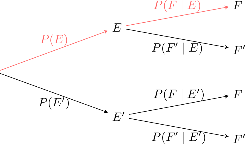
Definition Conditional Probability Tree Diagram
A conditional probability tree visually organizes probabilities for a sequence of events: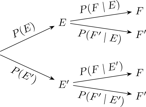
- Each branch shows a probability (e.g., \(P(E)\) or \(\PCond{F}{E}\)).
- Events are labeled at the end of each branch.
Un diagramme en arbre des probabilités conditionnelles organise visuellement les probabilités pour une suite d’événements :
- Chaque branche montre une probabilité (comme \(P(E)\) ou \(\PCond{F}{E}\)).
- Les événements sont marqués à la fin de chaque branche.
Example
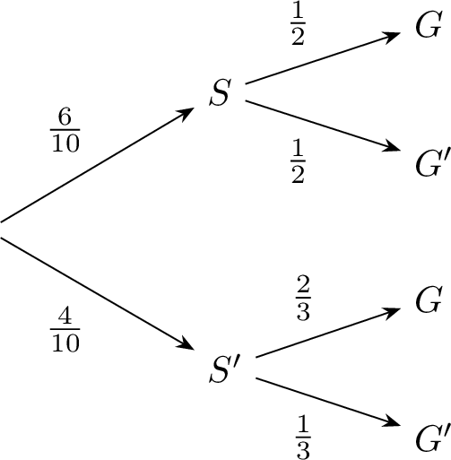
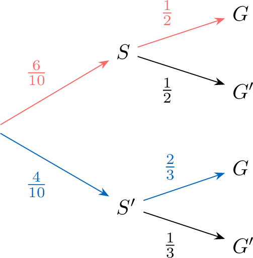
The probability Sam coaches a game is \(\frac{6}{10}\), and Alex coaches is \(\frac{4}{10}\). If Sam coaches, the chance a player is goalkeeper is \(\frac{1}{2}\); if Alex coaches, it’s \(\frac{2}{3}\).
Draw the tree diagram.
Draw the tree diagram.
- Define the events:
- \(S\): Sam coaches.
- \(G\): Player is goalkeeper.
- Define the probabilities:
- \(P(S) = \frac{6}{10}\) and \(P(S') =1 - P(S)= \frac{4}{10}\).
- \(\PCond{G}{S} = \frac{1}{2}\) and \(\PCond{G'}{S} = 1 - \PCond{G}{S} = \frac{1}{2}\)
- \(\PCond{G}{S'} = \frac{2}{3}\) and \(\PCond{G'}{S'} = 1-\PCond{G}{S'}= \frac{1}{3}\)
- Tree diagram:
Joint Probability: \(P(E \text{ and } F)\)
Sometimes we know \(P(E)\) and \(\PCond{F}{E}\) and need the chance both \(E\) and \(F\) happen together—like finding the odds a student is a girl who loves math.
Proposition Joint Probability Formula
$$P(E \text{ and } F) = P(E) \times \PCond{F}{E}, \quad P(E \text{ and } F) = P(F) \times \PCond{E}{F}.$$
Method Finding \(P(E \text{ and } F)\) in a Tree
- Identify the path where \(E\) and \(F\) both occur.
- Multiply the probabilities along that path.
Example
For this probability tree,
- Path: \(S\) to \(G\) (highlighted):
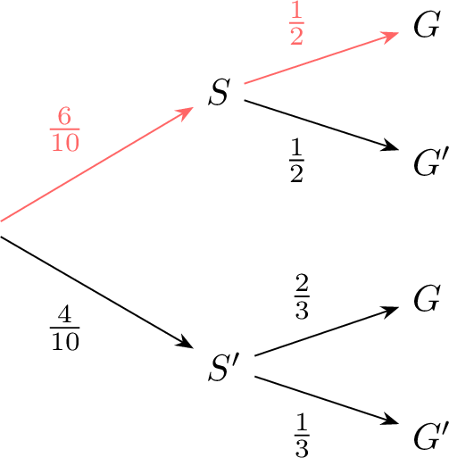
- Calculate:$$\begin{aligned}P(S \text{ and } G) &= P(S) \times \PCond{G}{S}\\ &= \frac{6}{10} \times \frac{1}{2}\\ &= \frac{3}{10}.\end{aligned}$$
Law of Total Probability
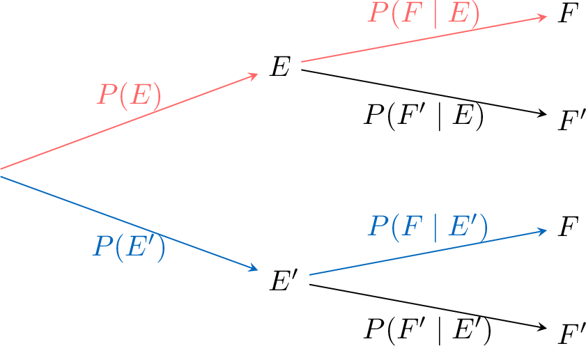
Theorem Law of Total Probability
For events \(E\) and \(F\):$$P(F) = P(E) \PCond{F}{E} + P(E') \PCond{F}{E'}.$$
Method Finding \(P(F)\) in a Tree
- Identify all paths to \(F\).
- Multiply probabilities along each path and sum them.
Example
For this probability tree,
- Paths to \(G\):
- Calculate:$$\begin{aligned}P(G) &= \textcolor{colordef}{\frac{6}{10} \times \frac{1}{2}} + \textcolor{colorprop}{\frac{4}{10} \times \frac{2}{3}} \\&= \textcolor{colordef}{\frac{6}{20}} + \textcolor{colorprop}{\frac{8}{30}} \\&= \textcolor{colordef}{\frac{9}{30}} + \textcolor{colorprop}{\frac{8}{30}} \\&= \textcolor{colordef}{\frac{17}{30}}.\end{aligned}$$
Bayes’ Theorem
What if you test positive for a rare disease—does that mean you have it? Bayes’ Theorem helps us flip conditional probabilities to answer questions like this, updating our beliefs with new evidence. It’s a cornerstone in fields like medicine and data science.
Theorem Bayes’ Theorem
$$\PCond{E}{F} = \frac{P(E) \PCond{F}{E}}{P(F)}, \quad \text{where } P(F) > 0.$$
Example
Consider a rare disease that affects approximately 1 in every 1,000 people. A medical test developed for detecting this disease has the following characteristics:
- Sensitivity: If a person has the disease, the test correctly returns a positive result 99\(\pourcent\) of the time.
- Specificity: If a person does not have the disease, the test correctly returns a negative result 95\(\pourcent\) of the time.
Define the following events clearly: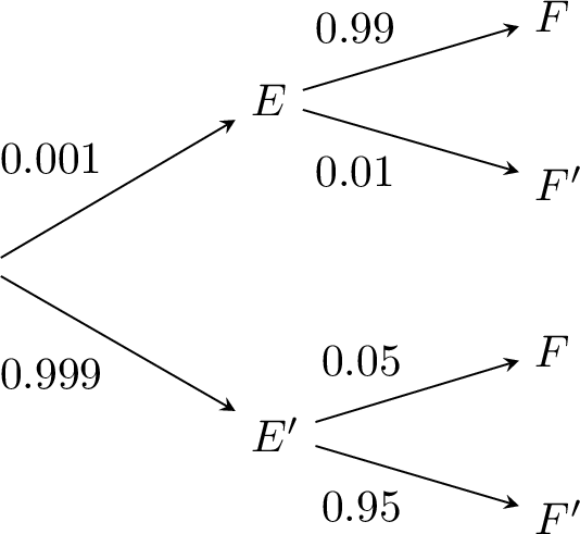
- Event \( E \): The person has the disease.
- Event \( F \): The test result is positive.
- \( P(E) = \frac{1}{1000} = 0.001 \), thus \( P(E') = 1 - 0.001 = 0.999 \).
- \( \PCond{F}{E} = 0.99 \), hence \( \PCond{F'}{E} = 1 - 0.99 = 0.01 \).
- \( \PCond{F'}{E'} = 0.95 \), hence \( \PCond{F}{E'} = 1 - 0.95 = 0.05 \).
Probability of Independent Events
Definition
Independent events are like you picking your favorite ice cream flavor while your friend chooses a movie—your decision doesn’t influence theirs, and theirs doesn’t affect yours!
Imagine rolling a die twice in a row. Define event \(E\) as getting an even number (like 2, 4, or 6) on the first roll, and event \(F\) as getting an odd number (like 1, 3, or 5) on the second roll. Here’s the key: knowing that \(E\) happened doesn’t change the chances of \(F\) occurring. In probability terms, the conditional probability of \(F\) given \(E\), written \(P_E(F)\), is the same as the probability of \(F\) alone, \(P(F)\).
Now, let’s connect this to joint probability. The chance of both \(E\) and \(F\) happening together, \(P(E \cap F)\), is given by$$ P(E \cap F) = P(E) \times \PCond{F}{E}.$$Since \(P_E(F) = P(F)\) for independent events, we can simplify this to:$$P(E \cap F) = P(E) \times P(F).$$This is the hallmark formula for independent events—a simple yet powerful idea that shows how some events can coexist without influencing each other!"
Definition Independent Events
Two events, \(E\) and \(F\), are independent if the chance of both happening is just the product of their individual chances. Mathematically:$$P(E \text{ and } F) = P(E) \times P(F)$$
Example
Imagine you do two totally separate actions:
- Flipping a fair coin (heads or tails).
- Rolling a fair six-sided die (1, 2, 3, 4, 5, or 6).
Let’s break it down:
- These events are independent, so we multiply their probabilities.
- For the coin: You’ve got two options—heads or tails—and they’re equally likely. So, \(P(\text{"tails"}) = \dfrac{1}{2}\).
- For the die: There are six sides, and “greater than 4” means 5 or 6. That’s 2 out of 6 possibilities, so \(P("\text{number} > 4") = \dfrac{2}{6}=\dfrac{1}{3}\).
- Now, combine them: $$\begin{aligned} P(\text{"tails" and "number} > 4") &= P(\text{"tails"}) \times P(\text{"number} > 4") \\ &= \dfrac{1}{2} \times \dfrac{1}{3} \\ &= \dfrac{1}{6} \end{aligned}$$
- Result: There’s a \(\dfrac{1}{6}\) chance of landing tails and rolling a 5 or 6.
Method Finding the probability of two independent events using a probability tree diagram
Let’s use a probability tree for our coin flip and die roll:
- Draw the Tree: Start with two branches for the coin: “Heads” and “Tails.” Then, from each, draw two more branches for the die: “Number > 4” (5 or 6) and “Number \(\leqslant\) 4” (1, 2, 3, or 4).
- Add Probabilities: Label each branch. The coin gives \(\dfrac{1}{2}\) for “Tails” and \(\dfrac{1}{2}\) for “Heads.” For the die, “Number > 4” is \(\dfrac{1}{3}\) (2 out of 6), and “Number \(\leqslant\) 4” is \(\dfrac{2}{3}\) (4 out of 6).
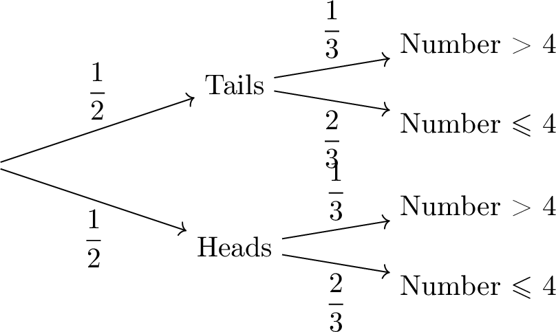
- Follow the Path: To find \(P(\text{tails and number} > 4)\), trace the “Tails” branch, then the “Number > 4” branch, and multiply: $$\dfrac{1}{2} \times \dfrac{1}{3} = \dfrac{1}{6}$$
- Wrap It Up: The tree confirms our answer—\(\dfrac{1}{6}\)!