Limits

Definition

The ancient Greek philosopher Zeno of Elea famously argued that motion was impossible. In his paradox of Achilles and the Tortoise, the swift hero Achilles can never overtake a slow tortoise given a head start, because by the time Achilles reaches the tortoise's starting point, the tortoise has already moved a little further ahead. When Achilles covers that new distance, the tortoise has moved ahead again. This process repeats endlessly, suggesting Achilles can never close the gap.
This paradox highlights a profound mathematical problem: how do we handle the infinitely small and the concept of "approaching" a value? It took mathematicians like Augustin-Louis Cauchy and Karl Weierstrass nearly two thousand years to formalize the answer with the concept of the limit. A limit describes the value a function "approaches" as its input gets closer and closer to a certain point. It is a foundational concept in calculus, because it underlies the definitions of both derivatives and integrals.

Definition Limit

A function $f$ has the limit $L$ as $x$ approaches $a$ if the values of $f(x)$ become arbitrarily close to the single real number $L$ whenever $x$ is sufficiently close to $a$ (but not necessarily equal to $a$), from both sides. We write this as:$$ \textcolor{colordef}{\lim_{x \to a} f(x) = L}\quad\text{or}\quad\textcolor{colordef}{f(x) \xrightarrow[x \to a]{} L}\quad\text{or}\quad\textcolor{colordef}{\text{as } x \to a,\ f(x)\to L}$$

The crucial idea of a limit is that it describes the behaviour of a function near a point, not at the point itself. The value of $f(a)$, or whether it even exists, is irrelevant to the value of the limit.
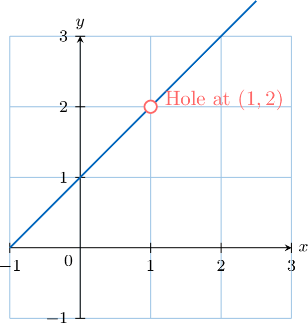
Consider the function $f(x) = \dfrac{x^2-1}{x-1}$. At $x=1$, the function is undefined. However, for any $x \neq 1$, we can simplify:$$ f(x) = \dfrac{(x-1)(x+1)}{x-1} = x+1. $$The graph of $f(x)$ is the line $y=x+1$ with a "hole" at $x=1$. As $x$ gets very close to 1 from either side, the value of $f(x)$ gets very close to 2. Therefore, $\displaystyle\lim_{x \to 1} f(x) = 2$, even though $f(1)$ is not defined.

Method Evaluating Limits

Direct Substitution: Always try substituting $x=a$ into the function first. If this gives a real number and the expression is defined (no division by zero, no square root of a negative, etc.), then that number is the limit.
Algebraic Manipulation: If substitution results in an indeterminate form like $\dfrac{0}{0}$, try to simplify the expression by:
- factoring and cancelling common factors;
- multiplying by a conjugate (for expressions with roots).
After simplifying, try direct substitution again.

Example

Evaluate $\displaystyle\lim_{x \to 2} x^2$.

Answer

We can evaluate the limit by direct substitution:$$\begin{aligned}\lim_{x \to 2} x^2 &= (2)^2 \\ &= 4\end{aligned}$$

Example

Evaluate $\displaystyle\lim_{x \to 0} \dfrac{x+x^2}{2x}$.

Answer

Direct substitution of $x=0$ results in the indeterminate form $\dfrac{0}{0}$. We must first simplify the expression algebraically for $x \neq 0$.$$\begin{aligned}\dfrac{x+x^2}{2x} &=\dfrac{x(1+x)}{2x} \\ &= \dfrac{1+x}{2}\quad (\text{for } x \neq 0) \\ &\xrightarrow[x \to 0]{}\dfrac{1+0}{2}= \dfrac{1}{2}\end{aligned}$$

Example

Evaluate $\displaystyle\lim_{x \to 1} \dfrac{\sqrt{x}-1}{x-1}$.

Answer

Direct substitution of $x=1$ results in the indeterminate form $\dfrac{\sqrt{1}-1}{1-1} = \dfrac{0}{0}$. Since the numerator involves a square root, we simplify by multiplying the numerator and the denominator by the conjugate of the numerator, which is $\sqrt{x}+1$.$$\begin{aligned}\dfrac{\sqrt{x}-1}{x-1} &= \left(\dfrac{\sqrt{x}-1}{x-1}\right) \cdot \left(\dfrac{\sqrt{x}+1}{\sqrt{x}+1}\right) \\ &= \dfrac{(\sqrt{x})^2 - 1^2}{(x-1)(\sqrt{x}+1)} && \text{(using }(a-b)(a+b)=a^2-b^2\text{)} \\ &= \dfrac{x-1}{(x-1)(\sqrt{x}+1)} \\ &= \dfrac{1}{\sqrt{x}+1} \quad (\text{for } x \neq 1)\\ &\xrightarrow[x \to 1]{} \dfrac{1}{\sqrt{1}+1} = \dfrac{1}{1+1} = \dfrac{1}{2}\end{aligned}$$

Algebraic Evaluation of Limits

While tables of values and graphs are useful for understanding the concept of a limit, they are not efficient for evaluation. Fortunately, limits follow a set of predictable algebraic rules, known as the Limit Laws, which allow us to calculate them directly.

Proposition The Limit Laws

Suppose that $c$ is a constant and the limits $\displaystyle\lim_{x \to a} f(x)$ and $\displaystyle\lim_{x \to a} g(x)$ both exist. Then:

Sum/Difference Law: $\displaystyle\lim_{x \to a} [f(x) \pm g(x)] = \displaystyle\lim_{x \to a} f(x) \pm \displaystyle\lim_{x \to a} g(x)$
Constant Multiple Law: $\displaystyle\lim_{x \to a} [c \cdot f(x)] = c \cdot \displaystyle\lim_{x \to a} f(x)$
Product Law: $\displaystyle\lim_{x \to a} [f(x) \cdot g(x)] = \left(\displaystyle\lim_{x \to a} f(x)\right) \cdot \left(\displaystyle\lim_{x \to a} g(x)\right)$
Quotient Law: $\displaystyle\lim_{x \to a} \dfrac{f(x)}{g(x)} = \dfrac{\displaystyle\lim_{x \to a} f(x)}{\displaystyle\lim_{x \to a} g(x)}$, provided $\displaystyle\lim_{x \to a} g(x) \neq 0$
Power Law: $\displaystyle\lim_{x \to a} [f(x)]^n = \left[\displaystyle\lim_{x \to a} f(x)\right]^n$, where $n$ is a positive integer.

These laws are the justification for using the Direct Substitution method on polynomials and on rational functions at points where the denominator is nonzero.

Example

Evaluate $\displaystyle\lim_{x \to 2} (3x^2 - 5x + 1)$ using the Limit Laws.

Answer

We apply the Limit Laws step by step:$$\begin{aligned}\displaystyle\lim_{x \to 2} (3x^2 - 5x + 1)&= \displaystyle\lim_{x \to 2} (3x^2) - \displaystyle\lim_{x \to 2} (5x) + \displaystyle\lim_{x \to 2} (1) && \text{(Sum/Difference Law)} \\ &= 3\left(\displaystyle\lim_{x \to 2} x^2\right) - 5\left(\displaystyle\lim_{x \to 2} x\right) + 1 && \text{(Constant Multiple Law)} \\ &= 3\left(\left[\displaystyle\lim_{x \to 2} x\right]^2\right) - 5(2) + 1 && \text{(Power Law)} \\ &= 3(2^2) - 10 + 1 && \text{(Direct Substitution)} \\ &= 12 - 10 + 1 = 3\end{aligned}$$This demonstrates that for any polynomial, the limit can be found by direct substitution, because polynomials are continuous everywhere.

Existence of a Limit

Definition One-Sided Limits

The right-hand limit, $\displaystyle\lim_{x \to a^+} f(x)$, is the value that $f(x)$ approaches as $x$ approaches $a$ from values greater than $a$.
The left-hand limit, $\displaystyle\lim_{x \to a^-} f(x)$, is the value that $f(x)$ approaches as $x$ approaches $a$ from values less than $a$.

Proposition Existence of a Limit

The two-sided limit $\displaystyle\lim_{x \to a} f(x)$ exists if and only if the left-hand and right-hand limits both exist and are equal:$$ \displaystyle\lim_{x \to a} f(x) = L \iff \displaystyle\lim_{x \to a^-} f(x) = L \text{ and } \displaystyle\lim_{x \to a^+} f(x) = L $$

Example

Consider the piecewise function $f(x) = \begin{cases} x, & x < 1 \\ x^2, & x \ge 1 \end{cases}$. Does $\lim_{x \to 1} f(x)$ exist?

Answer

To determine if the limit exists, we must find the left-hand and right-hand limits and check if they are equal.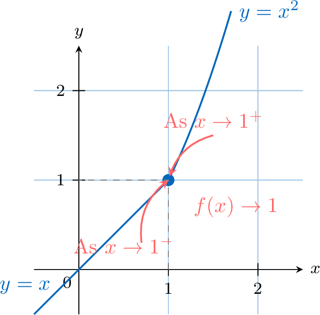

Left-hand limit: As $x \to 1^-$, we use the rule for $x<1$.$$ \lim_{x \to 1^-} f(x) = \lim_{x \to 1^-} (x) = 1 $$
Right-hand limit: As $x \to 1^+$, we use the rule for $x \ge 1$.$$ \lim_{x \to 1^+} f(x) = \lim_{x \to 1^+} (x^2) = 1^2 = 1 $$

Since the left-hand limit (1) is equal to the right-hand limit (1), the limit exists and $\lim_{x \to 1} f(x) = 1$.

Example

Consider the piecewise function $f(x) = \begin{cases} x+1, & x < 1 \\ x^2, & x \ge 1 \end{cases}$. Does $\lim_{x \to 1} f(x)$ exist?

Answer

To determine if the limit exists, we must find the left-hand and right-hand limits and check if they are equal.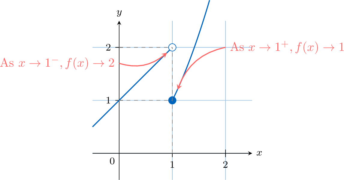

Left-hand limit: As $x \to 1^-$, we use the rule for $x<1$.$$ \lim_{x \to 1^-} f(x) = \lim_{x \to 1^-} (x+1) = 1+1 = 2 $$
Right-hand limit: As $x \to 1^+$, we use the rule for $x \ge 1$.$$ \lim_{x \to 1^+} f(x) = \lim_{x \to 1^+} (x^2) = 1^2 = 1 $$

Since the left-hand limit (2) is not equal to the right-hand limit (1), the limit $\lim_{x \to 1} f(x)$ does not exist. The graph shows a "jump" at $x=1$.

Infinite Limits and Vertical Asymptotes

We have seen that a limit fails to exist if the function approaches different values from the left and right. Another way a limit can fail to exist is if the function's values grow without bound, approaching positive or negative infinity. While these limits do not technically exist as finite numbers, we use limit notation as a precise way to describe this "unbounded behaviour," which corresponds to a vertical asymptote on a graph.

Definition Infinite Limit

The notation $\displaystyle\lim_{x \to a} f(x) = +\infty$ means that the values of $f(x)$ can be made arbitrarily large and positive by taking $x$ sufficiently close to $a$ (from both sides).
Similarly for $\displaystyle\lim_{x \to a} f(x) = -\infty$. In this situation we say that the limit diverges to $+\infty$ or $-\infty$; it is not a finite real number.

Definition Vertical Asymptote

The line $x=a$ is a vertical asymptote of the graph of the function $f(x)$ if the function approaches $+\infty$ or $-\infty$ as $x$ approaches $a$ from the left or the right.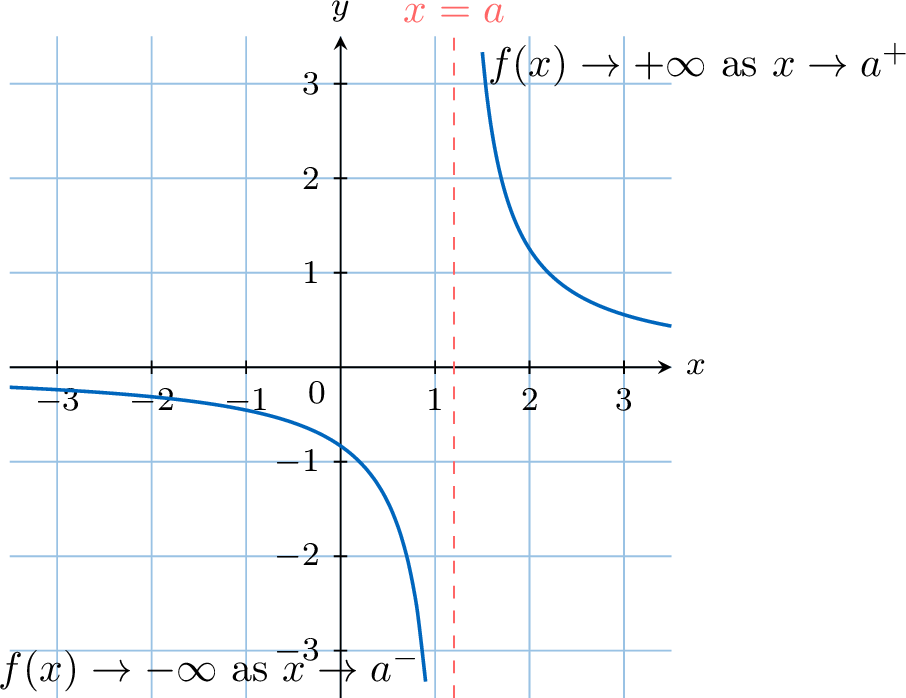

Example

Investigate $\displaystyle\lim_{x \to 0} \dfrac{1}{x^2}$.

Answer

Direct substitution of $x=0$ results in $\dfrac{1}{0}$, which is undefined, suggesting a vertical asymptote at $x=0$. We check the one-sided limits: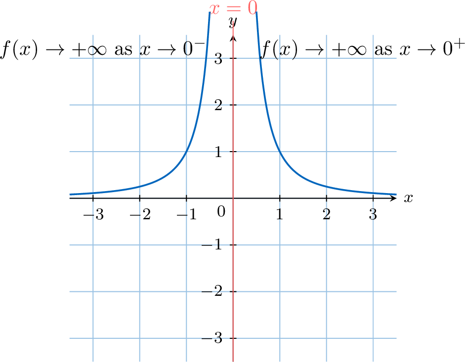

As $x \to 0^+$, $x^2$ is a small positive number, so $\dfrac{1}{x^2} \to +\infty$.
As $x \to 0^-$, $x^2$ is also a small positive number, so $\dfrac{1}{x^2} \to +\infty$.

Since the function's values increase without bound towards $+\infty$ from both sides, we describe this behavior as $\displaystyle\lim_{x \to 0} \dfrac{1}{x^2} = +\infty$.

Limits at Infinity

Limits at infinity describe the end behaviour of a function. When $\displaystyle\lim_{x \to \infty} f(x) = L$ (or $\displaystyle\lim_{x \to -\infty} f(x) = L$), the line $y=L$ is a horizontal asymptote of the graph.

Definition Limit at Infinity

A function $f$ has the limit $L$ as $x$ approaches $+\infty$ when the values of $f(x)$ become arbitrarily close to the single real number $L$ for all sufficiently large $x$. We write:$$ \textcolor{colordef}{\lim_{x \to +\infty} f(x) = L}\quad\text{or}\quad\textcolor{colordef}{f(x) \xrightarrow[x \to +\infty]{} L}. $$A similar definition applies for $x \to -\infty$.

Definition Horizontal Asymptote

The line $y=L$ is a horizontal asymptote of the graph of the function $f(x)$ if either of the following limit conditions is met:$$ \lim_{x \to \infty} f(x) = L \quad \text{or} \quad \lim_{x \to -\infty} f(x) = L $$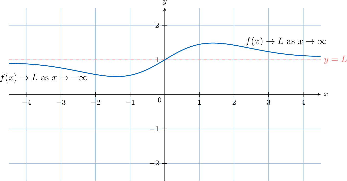

Example

Evaluate $\displaystyle\lim_{x \to \infty} \dfrac{3x^2 - x + 4}{2x^2 + 5x - 1}$.

Answer

First, we manipulate the expression by factoring out the highest power of $x$ from the numerator and the denominator, which is $x^2$.$$\begin{aligned}\dfrac{3x^2 - x + 4}{2x^2 + 5x - 1}&= \dfrac{x^2\left(3 - \frac{1}{x} + \frac{4}{x^2}\right)}{x^2\left(2 + \frac{5}{x} - \frac{1}{x^2}\right)} \\ &=\dfrac{3 - \frac{1}{x} + \frac{4}{x^2}}{2 + \frac{5}{x} - \frac{1}{x^2}} \quad \text{for } x \neq 0\end{aligned}$$Now, we can take the limit of the simplified expression as $x \to \infty$, using the fact that terms like $\frac{c}{x^n}$ approach $0$:$$ \lim_{x \to \infty} \dfrac{3 - \frac{1}{x} + \frac{4}{x^2}}{2 + \frac{5}{x} - \frac{1}{x^2}} = \dfrac{3 - 0 + 0}{2 + 0 - 0} = \dfrac{3}{2}. $$

The Squeeze Theorem

Some limits, particularly those involving oscillating functions like $\sin(1/x)$, cannot be evaluated using direct substitution or standard algebraic manipulation alone. For these cases, we may be able to use the Squeeze Theorem (also known as the Sandwich Theorem). The idea is to find two simpler functions that "squeeze" or "sandwich" the more complex function between them. If these two outer functions approach the same limit, then the function trapped in the middle must also approach that same limit.

Proposition The Squeeze Theorem

Suppose that for all $x$ in some interval around $a$ (except possibly at $x=a$):$$ g(x) \le f(x) \le h(x). $$And suppose that:$$ \lim_{x \to a} g(x) = \lim_{x \to a} h(x) = L. $$Then, we can conclude that:$$ \lim_{x \to a} f(x) = L. $$

Example

Evaluate $\displaystyle\lim_{x \to 0} x^2 \sin\left(\dfrac{1}{x}\right)$.

Answer

We cannot use direct substitution because $\sin(1/0)$ is undefined. The function $f(x) = x^2 \sin(1/x)$ is made of two parts: $x^2$, which approaches $0$, and $\sin(1/x)$, which oscillates infinitely between $-1$ and $1$ as $x \to 0$. This suggests using the Squeeze Theorem.
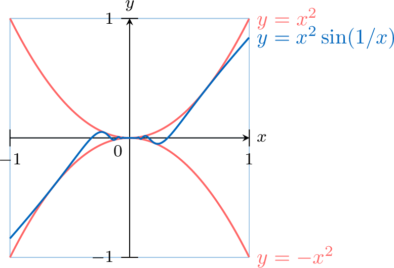
We start with the known range of the sine function:$$ -1 \le \sin\left(\dfrac{1}{x}\right) \le 1. $$Since $x^2 \ge 0$, we can multiply the entire inequality by $x^2$ without changing the direction of the inequality signs:$$ -x^2 \le x^2 \sin\left(\dfrac{1}{x}\right) \le x^2. $$We have now "squeezed" our function between $g(x)=-x^2$ and $h(x)=x^2$. Next, we find the limits of these outer functions as $x \to 0$:$$ \lim_{x \to 0} (-x^2) = 0 \quad \text{and} \quad \lim_{x \to 0} (x^2) = 0. $$Since our function is trapped between two functions that both approach the limit $0$, by the Squeeze Theorem, our limit must also be $0$:$$ \lim_{x \to 0} x^2 \sin\left(\dfrac{1}{x}\right) = 0. $$

Continuity

Definition Continuity at a Point

A function $f$ is continuous at a point $x=a$ if three conditions are met:

$f(a)$ is defined (the point exists).
$\displaystyle\lim_{x \to a} f(x)$ exists (the limit exists).
$\displaystyle\lim_{x \to a} f(x) = f(a)$ (the limit equals the function's value).

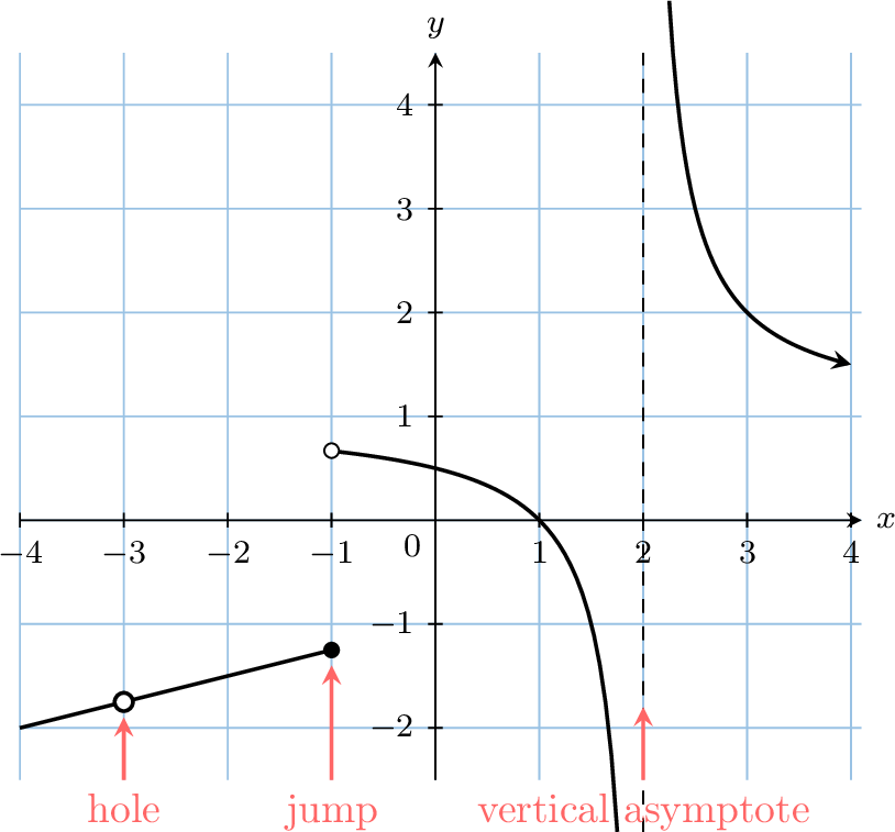
Intuitively, a function is continuous over an interval if its graph can be drawn without lifting your pen from the paper.

Types of Discontinuity

Removable Discontinuity: Occurs when the limit exists but is not equal to the function's value, or the function is not defined at the point. This corresponds to a "hole" in the graph. It can be "removed" by redefining the function at that single point.
Non-Removable (Essential) Discontinuity: Occurs when the limit does not exist. This corresponds to a "jump" (where one-sided limits differ), a vertical asymptote (an infinite discontinuity), or more complicated oscillatory behaviour.

Proposition A Catalog of Continuous Functions

The following types of functions are continuous at every number in their domains:

Polynomials (e.g., $f(x)=x^2-3x+5$)
Rational functions (e.g., $f(x)=\dfrac{x+1}{x-2}$, continuous for $x \neq 2$)
Root functions (e.g., $f(x)=\sqrt[n]{x}$, continuous on their domains)
Trigonometric functions (e.g., $\sin(x), \cos(x), \tan(x)$, etc., continuous on their domains)
Inverse trigonometric functions (e.g., $\arctan(x), \arcsin(x)$, etc.)
Exponential functions (e.g., $f(x)=a^x, a>0$)
Logarithmic functions (e.g., $f(x)=\log_a(x)$, continuous for $x>0$)

Furthermore, any sum, difference, product, or composition of these functions is also continuous on its domain.

Proposition Limit of a Composite Function

If $\displaystyle\lim_{x \to a} g(x) = L$ and if the function $f$ is continuous at $L$, then:$$ \lim_{x \to a} f(g(x)) = f\left(\lim_{x \to a} g(x)\right) = f(L). $$

In essence, if the outer function is continuous, you can "move the limit inside the function."

Example

Evaluate $\displaystyle\lim_{x \to \infty} \ln\left(\dfrac{x+1}{x}\right)$.

Answer

We apply the Limit of a Composite Function rule. Since the natural logarithm function is continuous for all positive inputs, we can move the limit inside the function:$$\begin{aligned}\lim_{x \to \infty} \ln\left(\dfrac{x+1}{x}\right)&= \ln\left(\lim_{x \to \infty} \dfrac{x+1}{x}\right) && (\text{since } \ln \text{ is continuous on } (0,\infty)) \\ &= \ln\left(\lim_{x \to \infty} \left(1+\frac{1}{x}\right)\right) && (\text{by algebraic simplification}) \\ &= \ln(1+0) \\ &= \ln(1) \\ &= 0.\end{aligned}$$