Exponential Functions
In previous chapters, we learned how to evaluate expressions like \(a^n\), where the exponent \(n\) was an integer or a rational number. This chapter extends that concept to the exponential function, written as \(f(x) = a^x\), where the exponent \(x\) can be any real number.
We will explore the key features and graphs of these functions and see how they are used to model real-world phenomena involving rapid growth or decay, such as population dynamics and compound interest.
We will explore the key features and graphs of these functions and see how they are used to model real-world phenomena involving rapid growth or decay, such as population dynamics and compound interest.
Exponential Functions
Definition Exponential Function
The exponential function has the form \(f(x)=a^x\), where the base \(a\) is a positive constant and \(a \neq 1\).
Proposition Key Features of the Graph of \(y\equal a^x\)
All exponential functions of the form \(f(x) = a^x\) share several key graphical features: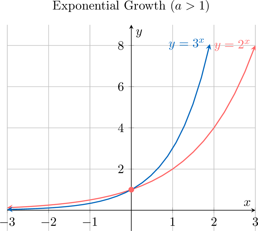 \(\quad\)
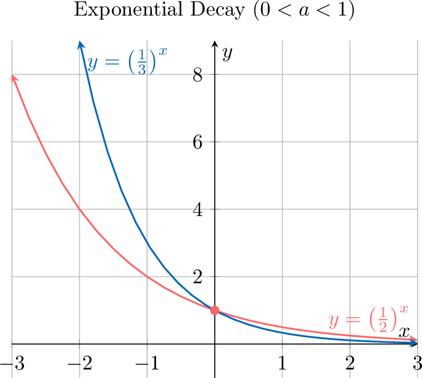
- Domain: The domain is all real numbers, \((-\infty, \infty)\).
- Range: The range is all positive real numbers, \((0, \infty)\).
- Horizontal Asymptote: The graph has a horizontal asymptote at the x-axis (\(y=0\)). The function approaches this line but never touches it.
- y-intercept: The graph always passes through the point \((0, 1)\), because \(a^0 = 1\) for any valid base \(a\).
- General Shape: The shape of the graph is determined by the value of the base, \(a\):
- If \(a > 1\), the function shows exponential growth and is increasing.
- If \(0 < a < 1\), the function shows exponential decay and is decreasing.
\(\quad\)Natural Exponential Function \(e^x\)
Definition Natural Exponential Function
The natural exponential function is \(x\mapsto e^x\).
- Domain: \((-\infty, +\infty)\)
- Range: \((0, +\infty)\)
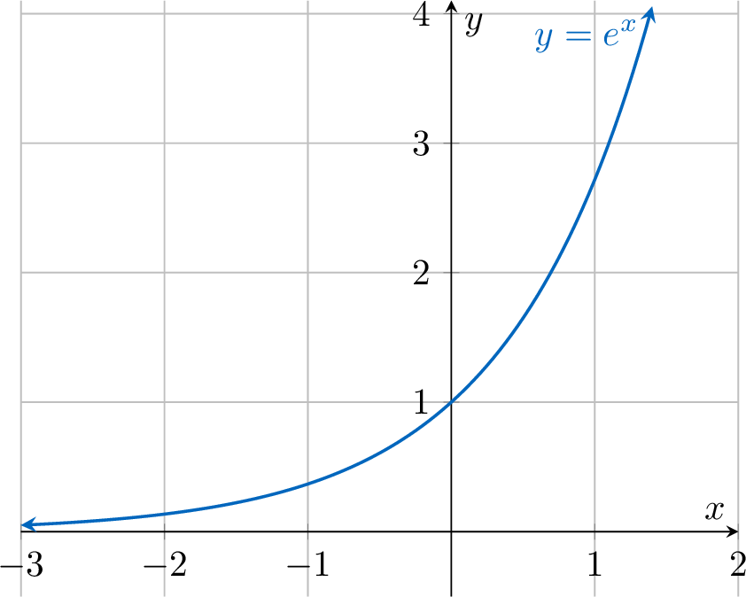
Proposition Graph and Properties of \(y\equal e^x\)
- Horizontal Asymptote: The graph has a horizontal asymptote at the x-axis (\(y=0\)) as \(x \to -\infty\).
- y-intercept: The graph passes through the point \((0, 1)\), since \(e^0 = 1\).
- It is a strictly increasing function.
Transformations of Exponential Functions
Proposition Transformations of Exponential Functions
The graph of the general exponential function \(f(x) = k \cdot a^{m(x-h)} + v\) can be obtained by applying transformations to the basic graph of \(y=a^x\).
- Vertical Translation (\(v\)): The graph is shifted up by \(v\) units. The horizontal asymptote becomes \(y=v\).
- Horizontal Translation (\(h\)): The graph is shifted to the right by \(h\) units.
- Vertical Stretch/Reflection (\(k\)): The graph is stretched vertically by a factor of \(|k|\). If \(k<0\), the graph is reflected in the horizontal asymptote.
- Horizontal Stretch/Reflection (\(m\)): The graph is stretched horizontally by a factor of \(1/|m|\) about the line \(x=h\). If \(m<0\), it is reflected across the vertical line \(x=h\) (across the \(y\)-axis only when \(h=0\)).
Example
Sketch the graph of \(f(x) = 2e^{-x} + 3\). State the domain, range, and equation of the asymptote.
The graph is a transformation of \(y=e^x\):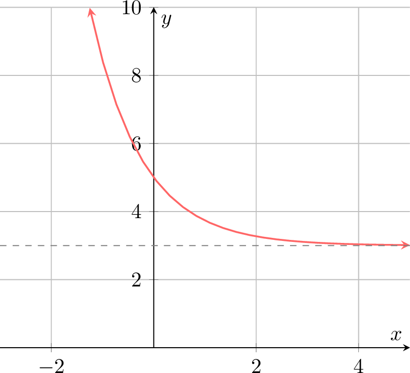
- Reflection in the y-axis (due to the negative in front of \(x\)).
- Vertical stretch by a factor of 2.
- Vertical shift 3 units up.
- The horizontal asymptote is \(\boldsymbol{y=3}\).
- The domain is \(\boldsymbol{\mathbb{R}}\).
- The range is \(\boldsymbol{(3, \infty)}\).
Exponential Models
Exponential functions are used to model quantities that change by a constant multiplicative factor over equal intervals of time. This core principle distinguishes them from linear functions, which change by a constant difference (addition or subtraction).
There are two main types of exponential models:
There are two main types of exponential models:
- Exponential Growth: The quantity increases by a constant factor greater than 1. This is seen in phenomena like population growth and compound interest.
- Exponential Decay: The quantity decreases by a constant factor between 0 and 1. This is seen in phenomena like radioactive decay and asset depreciation.
Definition General Model for Exponential Growth and Decay
An exponential relationship is described by the function:$$ A(t) = A_0 \times R^t $$where:
- \(A(t)\) is the amount at time \(t\).
- \(A_0\) is the initial amount (the amount at \(t=0\)).
- \(R\) is the constant growth or decay factor per unit of time.
- \(t\) is the time elapsed.
Example
The population of foxes, \(P\), in a specified area, \(t\) years after observation began, is modeled by the equation: \(P(t)=300(1.25)^t\).
- How many foxes are there initially?
- What is the annual percentage growth rate?
- How many foxes are there after 5 years?
- The initial population corresponds to \(t=0\). $$P(0) = 300(1.25)^0 = 300 \times 1 = \boldsymbol{300} \text{ foxes}$$
- The growth factor is \(R=1.25\). Since \(R = 1+r\), we have \(1.25 = 1+r\), which gives \(r=0.25\).
The annual growth rate is \(\boldsymbol{25\pourcent}\). - Substitute \(t=5\) into the equation. Since the population must be a whole number, we round to the nearest fox. $$P(5) = 300(1.25)^5 \approx 915.52... \approx \boldsymbol{916} \text{ foxes}$$
Example
An amount of \(\dollar 5\,000\) is invested at \(6\pourcent\) p.a. compounded annually.
- Find a model for the amount, \(A\), after \(t\) years.
- Find the amount after 4 years.
- The initial amount is \(A_0 = 5\,000\). The annual interest rate is \(r = 0.06\).
The growth factor is \(R = 1+r = 1+0.06 = 1.06\).
The model is \(\boldsymbol{A(t) = 5\,000(1.06)^t}\). - After 4 years, the amount is: $$A(4) = 5\,000(1.06)^4 \approx 6\,312.38...$$ The amount is \(\boldsymbol{\dollar 6\,312.38}\).