Continuity
Definition
Definition Continuity at a Point
A function \(f\) is continuous at a point \(x=a\) if three conditions are met:
- \(f(a)\) is defined (the point exists).
- \(\displaystyle\lim_{x \to a} f(x)\) exists (the limit exists).
- \(\displaystyle\lim_{x \to a} f(x) = f(a)\) (the limit equals the function's value).
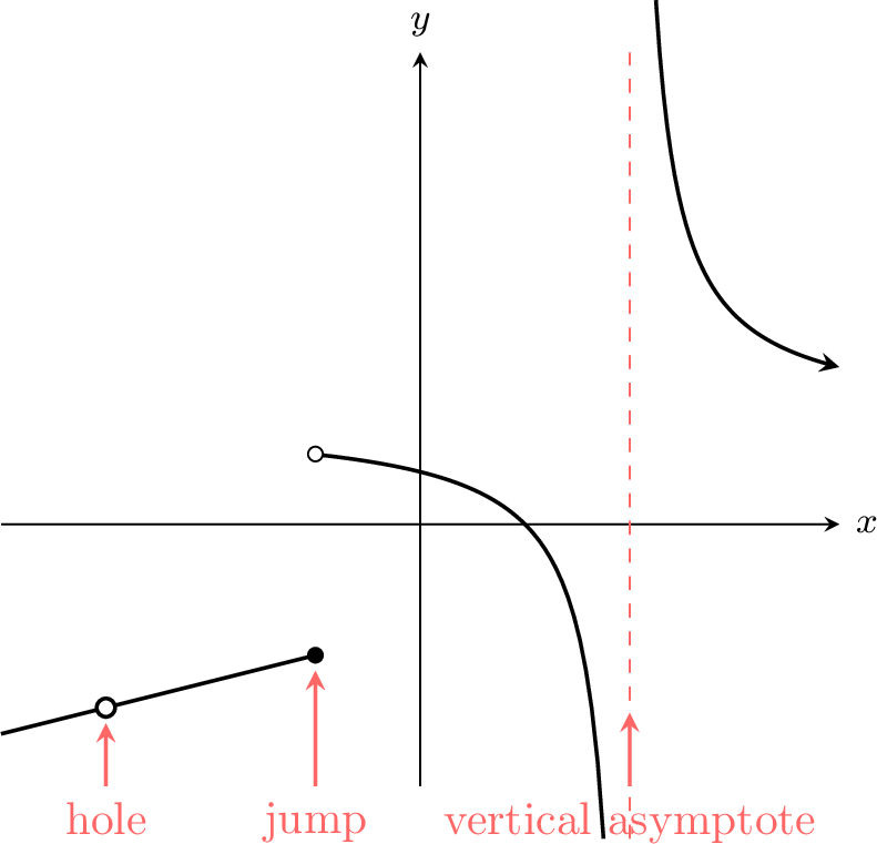
Types of Discontinuity
- Removable Discontinuity: Occurs when the limit exists but is not equal to the function's value, or the function is not defined at the point. This corresponds to a "hole" in the graph. It can be "removed" by redefining the function at that single point.
- Non-Removable (Essential) Discontinuity: Occurs when the limit does not exist. This corresponds to a "jump" (where one-sided limits differ), a vertical asymptote (an infinite discontinuity), or more complicated oscillatory behaviour.
Proposition A Catalog of Continuous Functions
The following types of functions are continuous at every number in their domains:
- Polynomials (e.g., \(f(x)=x^2-3x+5\))
- Rational functions (e.g., \(f(x)=\dfrac{x+1}{x-2}\), continuous for \(x \neq 2\))
- Root functions (e.g., \(f(x)=\sqrt[n]{x}\), continuous on their domains)
- Trigonometric functions (e.g., \(\sin(x), \cos(x), \tan(x)\), etc., continuous on their domains)
- Inverse trigonometric functions (e.g., \(\arctan(x), \arcsin(x)\), etc.)
- Exponential functions (e.g., \(f(x)=e^x\))
- Natural logarithm (e.g., \(f(x)=\ln(x)\), continuous for \(x>0\))
Limit of a Composite Function
Proposition Limit of a Composite Function
If \(\displaystyle\lim_{x \to a} g(x) = L\) and if the function \(f\) is continuous at \(L\), then:$$ \lim_{x \to a} f(g(x)) = f\left(\lim_{x \to a} g(x)\right) = f(L). $$
In essence, if the outer function is continuous, you can "move the limit inside the function."
Example
Evaluate \(\displaystyle\lim_{x \to \infty} \ln\left(\dfrac{x+1}{x}\right)\).
We apply the Limit of a Composite Function rule. Since the natural logarithm function is continuous for all positive inputs, we can move the limit inside the function:$$\begin{aligned}\lim_{x \to \infty} \ln\left(\dfrac{x+1}{x}\right)&= \ln\left(\lim_{x \to \infty} \dfrac{x+1}{x}\right) && (\text{since } \ln \text{ is continuous on } (0,\infty)) \\
&= \ln\left(\lim_{x \to \infty} \left(1+\frac{1}{x}\right)\right) && (\text{by algebraic simplification}) \\
&= \ln(1+0) \\
&= \ln(1) \\
&= 0.\end{aligned}$$
Continuity and Differentiability
Theorem Continuity and Differentiability
If a function \(f\) is differentiable at a point \(a\), then \(f\) is continuous at \(a\).
If a function \(f\) is differentiable on an interval \(I\), then \(f\) is continuous on \(I\).
If a function \(f\) is differentiable on an interval \(I\), then \(f\) is continuous on \(I\).
Note
The converse of this theorem is false. A function can be continuous at a point without being differentiable there.
The classic example is the absolute value function \(f(x) = |x|\) at \(x=0\):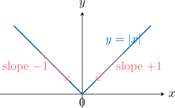
The classic example is the absolute value function \(f(x) = |x|\) at \(x=0\):
- It is continuous at 0 because \(\displaystyle\lim_{x \to 0} |x| = 0 = f(0)\).
- It is not differentiable at 0 because the slope on the left is \(-1\) and the slope on the right is \(+1\).
Continuity and Sequences
Theorem Fixed Point Theorem
Let \((u_n)\) be a sequence defined by \(u_{n+1} = f(u_n)\) that converges to a limit \(\ell\).
If the function \(f\) is continuous at \(\ell\), then the limit \(\ell\) is a solution to the equation:$$ f(x) = x $$
If the function \(f\) is continuous at \(\ell\), then the limit \(\ell\) is a solution to the equation:$$ f(x) = x $$
Note
- The continuity of \(f\) at \(\ell\) is essential for this theorem to hold.
- In practice, we solve \(f(x)=x\) to find potential limits and then use sequence properties to determine which one is correct.
Continuity and Equations
Theorem Intermediate Value Theorem (IVT)
Let \(f\) be a continuous function on an interval \([a, b]\).
For every real number \(k\) between \(f(a)\) and \(f(b)\), there exists at least one solution \(c\) in the interval \([a, b]\) such that:$$ f(c) = k $$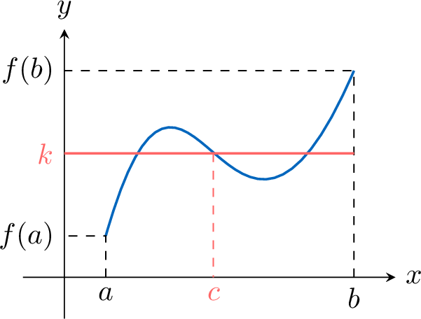
For every real number \(k\) between \(f(a)\) and \(f(b)\), there exists at least one solution \(c\) in the interval \([a, b]\) such that:$$ f(c) = k $$
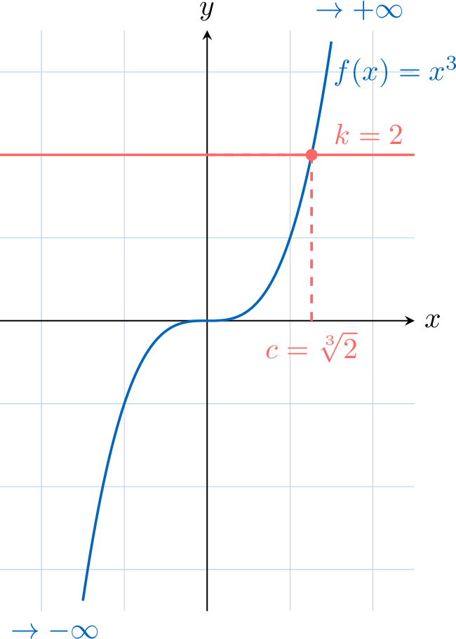
Theorem Corollary: Bijection Theorem
If \(f\) is continuous and strictly monotonic (always increasing or always decreasing) on \([a, b]\), then for every \(k\) between \(f(a)\) and \(f(b)\), the equation \(f(x) = k\) has a unique solution \(c\) in \([a, b]\).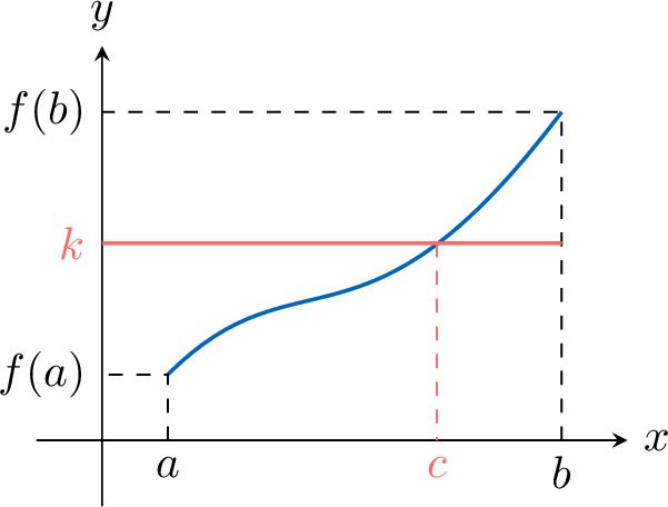
Example
The equation \(x^3 = 2\) has a unique solution on \(]-\infty, +\infty[\) because the function \(f(x) = x^3\) is continuous and strictly increasing on \(\mathbb{R}\), and 2 is between \(\displaystyle\lim_{x \to -\infty} x^3 = -\infty\) and \(\displaystyle\lim_{x \to +\infty} x^3 = +\infty\).