Continuous Random Variables

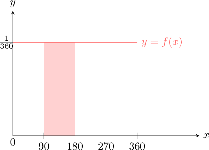
Consider a random experiment where a spinner is spun, and the continuous random variable $X$ represents the angle spun, measured in degrees over the interval $[0, 360)$.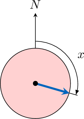

The probability that $X$ assumes any precise value, such as $x = 125.333\ldots$, is zero due to the infinite number of possible outcomes within a continuous range. However, we can calculate the probability that $X$ lies within an interval, such as $[90, 180]$, by summing the probabilities over tiny subintervals within this range:$$\begin{aligned}P(90 \leq X \leq 180) &= \sum_{x \in [90, 180]} P(x \leq X < x + dx) \\&= \sum_{x \in [90, 180]} \frac{P(x \leq X < x + dx)}{dx} \cdot dx\end{aligned}$$We define the probability density function, $f(x) = \frac{P(x \leq X < x + dx)}{dx}$, as the probability per unit length. By the definition of integration, this summation becomes:$$P(90 \leq X \leq 180) = \int_{90}^{180} f(x) \, dx$$For a uniform spinner, the probability is evenly distributed across all angles, so the pdf is constant: $f(x) = \frac{1}{360}$ for $x \in [0, 360)$. Thus:$$\begin{aligned}P(90 \leq X \leq 180) &= \int_{90}^{180} \frac{1}{360} \, dx \\&= \left[ \frac{x}{360} \right]_{90}^{180} \\&= \frac{180}{360} - \frac{90}{360} \\&= \frac{1}{4}\end{aligned}$$Hence, the probability of spinning an angle between 90 and 180 degrees is $\frac{1}{4}$.

Definitions

Probability Density Function

A probability density function describes the likelihood of a continuous random variable taking values within a specific range. Unlike discrete random variables, where probabilities are assigned to individual outcomes, continuous variables use the pdf to compute probabilities over intervals via integration.

Definition Probability Density Function

A function $f$ is a probability density function (pdf) on the interval $[a, b]$ if:

$f(x) \geq 0$ for all $x \in [a, b]$ (non-negative everywhere),
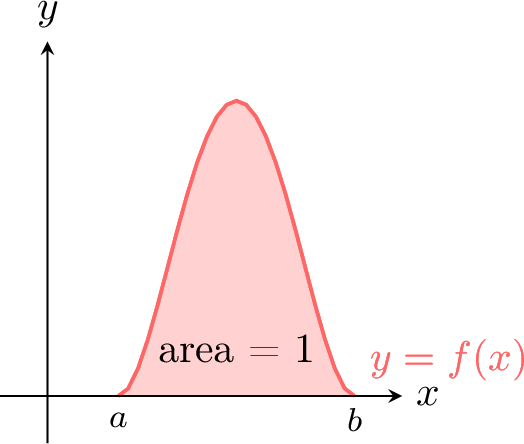
$\int_{a}^{b} f(x) \, dx = 1$ (the total area under the curve equals 1).

Example

The random variable $X$ takes values on $[0, 2]$ with density $f(x) = \frac{x}{2}$.

Verify that $f$ is a probability density function on $[0, 2]$.

Answer

$f(x) = \frac{x}{2} \geq 0$ for all $x \in [0, 2]$, since $x \geq 0$.
Compute the total area: $$ \begin{aligned}[t] \int_{0}^{2} f(x) \, dx &= \int_{0}^{2} \frac{x}{2} \, dx \\ &= \left[ \frac{x^2}{4} \right]_{0}^{2} \\ &= \frac{2^2}{4} - 0 = 1 \end{aligned} $$ Since both conditions hold, $f(x) = \frac{x}{2}$ is a valid pdf on $[0, 2]$.

Definition Density of a Continuous Random Variable

A random variable $X$ with values on $[a, b]$ has a density $f$, if the probability that $X$ lies between $c$ and $d$ ($c, d \in [a, b]$) is:$$P(c \leq X \leq d) = \int_{c}^{d} f(x) \, dx$$This represents the area under the curve $y = f(x)$ from $x = c$ to $x = d$.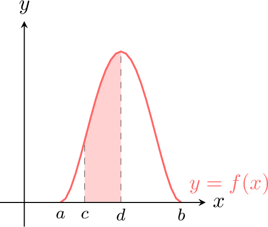

Remark

Since $f(x) \geq 0$, $P(c \leq X \leq d) \geq 0$.
Since $\int_{a}^{b} f(x) \, dx = 1$, $P(a \leq X \leq b) = 1$.

Example

The random variable $X$ with values on $[0, 2]$ has density $f(x) = \frac{x}{2}$. Find $P(1 \leq X \leq 2)$.

Answer

$$\begin{aligned}[t]P(1 \leq X \leq 2) &= \int_{1}^{2} \frac{x}{2} \, dx \\&= \left[ \frac{x^2}{4} \right]_{1}^{2} \\&= \frac{2^2}{4} - \frac{1^2}{4} \\&= 1 - \frac{1}{4}\\&= \frac{3}{4}\end{aligned}$$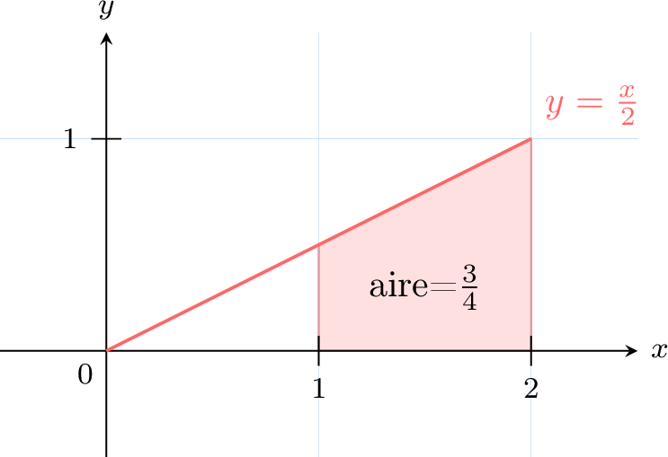

Expectation

The expectation (or expected value) of a continuous random variable is the "average" value it would take if the experiment were repeated infinitely. It represents the center of the distribution and is calculated as a discrete random variable:$$\begin{aligned}[t]E(X)&=\sum_{x\in[a,b]}x P(x \leqslant X < x+\mathrm d x)\\&=\sum_{x\in[a,b]}x \dfrac{P(x \leqslant X < x+\mathrm d x)}{\mathrm d x}\mathrm d x\\&=\int_{a}^b xf(x)\;\mathrm d x\\\end{aligned}$$

Definition Expectation

For a continuous random variable $X$ with density $f$ on $[a, b]$, the expected value is $$E(X) = \int_{a}^{b} x f(x) \, dx.$$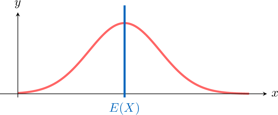

Example

The random variable $X$ with values on $[0, 3]$ has density $f(x) = \frac{x^2}{9}$: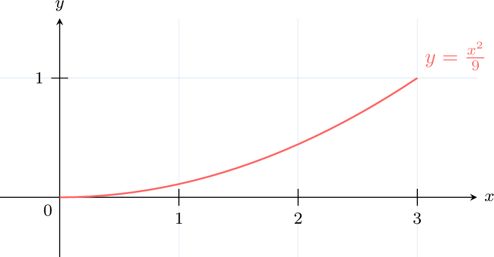

Find $E(X)$.

Answer

Compute $E(X)$: $$ \begin{aligned}[t] E(X) &= \int_{0}^{3} x \cdot \frac{x^2}{9} \, dx \\ &= \int_{0}^{3} \frac{x^3}{9} \, dx \\ &= \left[ \frac{x^4}{36} \right]_{0}^{3} \\ &= \frac{3^4}{36} - 0 \\ &= 2.25 \end{aligned} $$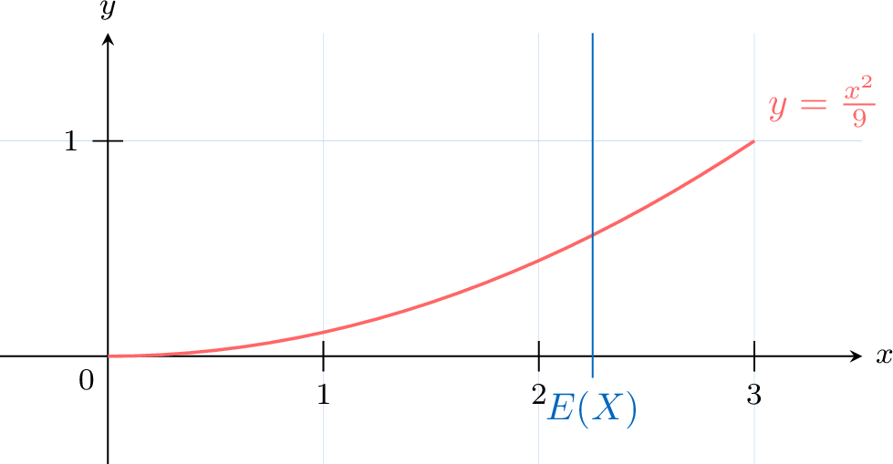

Example

The random variable $X$ with values on $[0, 2]$ has density $f(x) = \frac{x}{2}$: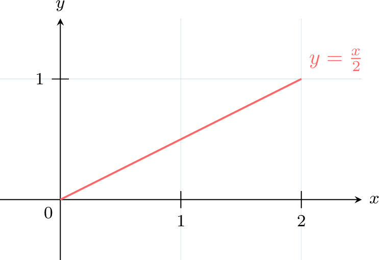

Find $E(X)$.

Answer

Compute $E(X)$:$$\begin{aligned}[t]E(X) &= \int_{0}^{2} x \cdot \frac{x}{2} \, dx \\&= \int_{0}^{2} \frac{x^2}{2} \, dx \\&= \left[ \frac{x^3}{6} \right]_{0}^{2} \\&= \frac{2^3}{6} - 0 \\&= \frac{8}{6} \\&= \frac{4}{3} \\\end{aligned}$$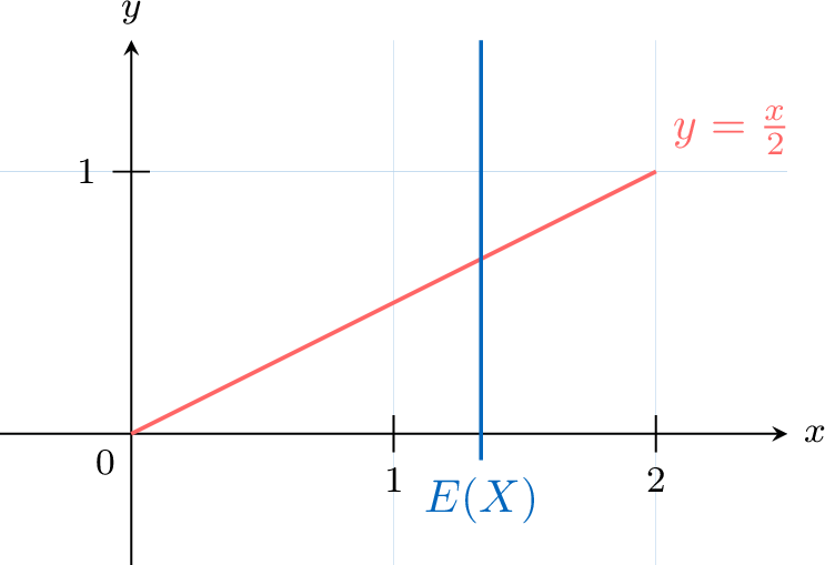

Variance

The variance of a continuous random variable measures the spread of its values around the expected value if the experiment were repeated infinitely. It quantifies the distribution’s dispersion and can be calculated as a discrete random variable:$$\begin{aligned}[t]V(X) &= \sum_{x \in [a, b]} (x - E(X))^2 P(x \leq X < x + dx) \\&= \sum_{x \in [a, b]} (x - E(X))^2 \frac{P(x \leq X < x + dx)}{dx} \cdot dx \\&= \int_{a}^{b} (x - E(X))^2 f(x) \, dx\end{aligned}$$

Definition Variance and Standard Deviation

For a continuous random variable $X$ with density $f$ on $[a, b]$, the variance is$$V(X) = \int_{a}^{b} (x - E(X))^2 f(x) \, dx.$$The standard deviation is$$\sigma = \sqrt{V(X)}.$$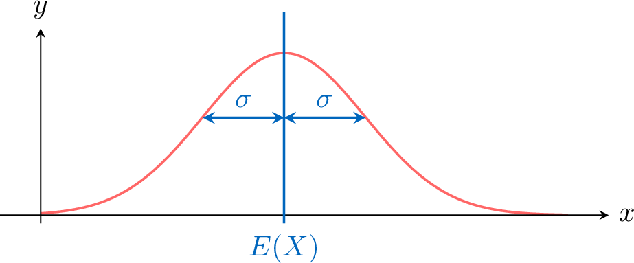

Proposition

An alternative formula for variance is:$$V(X) = \int_{a}^{b} x^2 f(x) \, dx - [E(X)]^2$$

Example

The random variable $X$ with values on $[0, 2]$ has density $f(x) = \frac{x}{2}$.
Find $V(X)$.

Answer

Compute $E(X)$: $$ \begin{aligned}[t] E(X) &= \int_{0}^{2} x \cdot \frac{x}{2} \, dx \\ &= \int_{0}^{2} \frac{x^2}{2} \, dx \\ &= \left[ \frac{x^3}{6} \right]_{0}^{2} \\ &= \frac{2^3}{6} - 0 \\ &= \frac{8}{6} \\ &= \frac{4}{3} \\ \end{aligned} $$
Compute $\int_{0}^{2} x^2 \cdot f(x) \, dx$: $$ \begin{aligned}[t] \int_{0}^{2} x^2 \cdot f(x) \, dx &=\int_{0}^{2} x^2 \cdot \frac{x}{2} \, dx\\ &= \int_{0}^{2} \frac{x^3}{2} \, dx \\ &= \left[ \frac{x^4}{8} \right]_{0}^{2} \\ &= \frac{2^4}{8} - 0 \\ &= \frac{16}{8} \\ &= 2 \end{aligned} $$
Compute $V(X)$ using the alternative formula: $$ \begin{aligned}[t] V(X) &= \int_{0}^{2} x^2 \cdot f(x) \, dx - [E(X)]^2 \\ &= 2 - \left(\frac{4}{3}\right)^2 \\ &= 2 - \frac{16}{9} \\ &= \frac{18}{9} - \frac{16}{9} \\ &= \frac{2}{9} \end{aligned} $$

Continuous Uniform Distribution

The continuous uniform distribution applies to events that are equally likely across an interval, such as the spinner example. The density is constant over the range.

Definition Continuous Uniform Distribution

A continuous random variable $X$ follows a continuous uniform distribution on $[a, b]$ if its density is:$$f(x) = \frac{1}{b - a} \quad \text{for} \quad a \leq x \leq b$$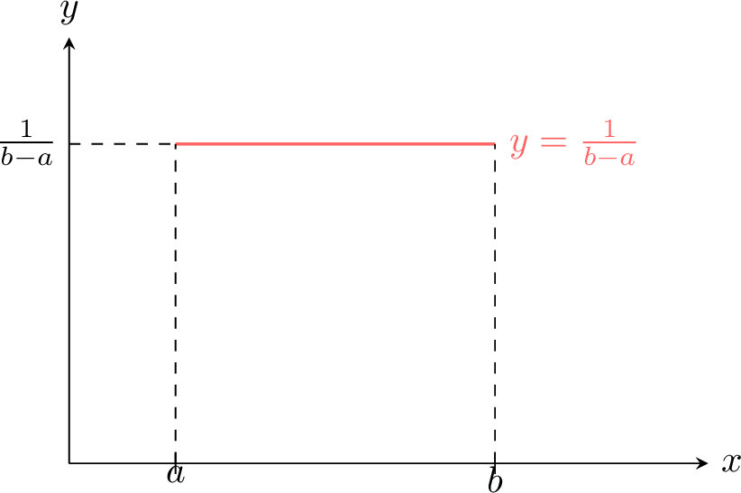

Proposition Properties

Let $ X $ be a continuous random variable following a continuous uniform distribution on $[a, b]$:

for all $ c, d \in [a, b] : P(c \leq X \leq d) = \frac{d - c}{b - a}$,
$E(X) = \frac{a + b}{2}$.

Proof

Probability: $$ \begin{aligned}[t] P(c \leq X \leq d) &= \int_{c}^{d} \frac{1}{b - a} \, dx \\ &= \left[ \frac{x}{b - a} \right]_{c}^{d} \\ &= \frac{d - c}{b - a} \end{aligned} $$
Expected value: $$ \begin{aligned}[t] E(X) &= \int_{a}^{b} x \cdot \frac{1}{b - a} \, dx \\ &= \left[ \frac{x^2}{2(b - a)} \right]_{a}^{b} \\ &= \frac{b^2 - a^2}{2(b - a)} = \frac{(b - a)(b + a)}{2(b - a)} = \frac{a + b}{2} \end{aligned} $$

Normal Distribution

The normal distribution is a key continuous distribution in statistics, often used to model real-world phenomena (e.g., heights, test scores) due to the Central Limit Theorem. This theorem states that the sum or average of many independent random variables, under certain conditions, approximates a normal distribution as the sample size increases. The normal curve is bell-shaped, symmetric, and centered at its mean.
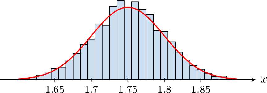
For example, we plot a histogram of the heights of boys at the university. The distribution represented by the histogram follows a bell-shaped curve, also known as a normal distribution.

Standard Normal Distribution

Definition Standard Normal Distribution

A continuous random variable $X$ follows a standard normal distribution (or $Z$-distribution) if its density is:$$f(x) = \frac{1}{\sqrt{2\pi}} e^{-\frac{x^2}{2}}, \quad -\infty < x < \infty$$The probability over an interval is:$$P(a \leq X \leq b) = \int_{a}^{b} \frac{1}{\sqrt{2\pi}} e^{-\frac{x^2}{2}} \, dx$$This is denoted $X \sim \mathcal{N}(0, 1)$.

Remark

The total probability is 1:$$\int_{-\infty}^{\infty} \frac{1}{\sqrt{2\pi}} e^{-\frac{x^2}{2}} \, dx = 1$$This is the area under the entire curve.

Normal Distribution

Definition Normal Distribution

A continuous random variable $X$ follows a normal distribution if its density is:$$f(x) = \frac{1}{\sigma \sqrt{2\pi}} e^{-\frac{1}{2} \left( \frac{x - \mu}{\sigma} \right)^2}, \quad -\infty < x < \infty$$where $\mu$ is the mean and $\sigma^2$ is the variance. The graph is a normal curve (bell-shaped), denoted $X \sim \mathcal{N}(\mu, \sigma^2)$.

Proposition Expectation and Variance

For $X \sim \mathcal{N}(\mu, \sigma^2)$:

$E(X) = \mu$,
$V(X) = \sigma^2$.

Proposition Coverage Probabilities

For $X \sim \mathcal{N}(\mu, \sigma^2)$:

$P(\mu - \sigma \leq X \leq \mu) = P(\mu \leq X \leq \mu + \sigma) \approx 34.13\pourcent$,
$P(\mu - 2\sigma \leq X \leq \mu - \sigma) = P(\mu + \sigma \leq X \leq \mu + 2\sigma) \approx 13.59\pourcent$,
$P(\mu - 3\sigma \leq X \leq \mu - 2\sigma) = P(\mu + 2\sigma \leq X \leq \mu + 3\sigma) \approx 2.15\pourcent$,
$P(X \leq \mu - 3\sigma) = P(\mu + 3\sigma \leq X) \approx 0.13\pourcent$.

$P(\mu - \sigma \leq X \leq \mu) \approx 34.13\pourcent$ means about 34.13$\pourcent$ of values lie between $\mu - \sigma$ and $\mu$.
Probabilities are additive: $P(\mu - \sigma \leq X \leq \mu + \sigma) \approx 34.13\pourcent + 34.13\pourcent = 68.26\pourcent$.

Example

Students’ heights at a school are normally distributed with mean $\mu = 172 \, \text{cm}$ and standard deviation $\sigma = 8 \, \text{cm}$.

Find the percentage of students with heights between 164 cm and 172 cm.
Find the percentage between 164 cm and 180 cm.
Find the percentage with heights above 196 cm.
Find the percentage with heights below 196 cm.
In a group of 500 students, how many are expected to have heights between 164 cm and 180 cm?

Answer

$P(164 \leq X \leq 172) = P(\mu - \sigma \leq X \leq \mu) = 34.13\pourcent$.
$P(164 \leq X \leq 180) = P(\mu - \sigma \leq X \leq \mu + \sigma) = 34.13\pourcent + 34.13\pourcent = 68.26\pourcent$.
$P(X > 196) = P(X \geq \mu + 3\sigma) = 0.13\pourcent$.
$P(X < 196) = 1 - P(X \geq 196) = 100\pourcent - 0.13\pourcent = 99.87\pourcent$.
Expected number = $68.26\pourcent \times 500 = 0.6826 \times 500 \approx 341$ students.

Quantile

Definition Quantile

The value $x$ such that $P(X \leq x) = 0.95$ is the 95$\pourcent$-quantile, meaning 95$\pourcent$ of the distribution lies below $x$.

Example

$X \sim \mathcal{N}(7, 2^2)$. Find the 95$\pourcent$-quantile.

Answer

Using a calculator (e.g., inverse normal function), for $P(X \leq x) = 0.95$ with $\mu = 7$ and $\sigma = 2$, we find $x \approx 10.29$.